
The Bike Sharing Demand problem requires using historical data on weather conditions and bicycle rental to predict the number of occupied bicycles (rentals) for a certain hour of a certain day.
In the original problem statement, there are 11 features available. The feature set contains both real, categorical, and binary data. For the demonstration, a training sample bike_sharing_demand.csv is used from the original data.
See the Bike Sharing Demand, part 1 of the task where we performed some initial problem analysis.
import warnings
warnings.filterwarnings("ignore")
from sklearn import model_selection, linear_model, metrics, pipeline, preprocessing
import numpy as np
import pandas as pd
%pylab inline
raw_data = pd.read_csv("bike_sharing_demand.csv", header = 0, sep = ",")
raw_data.head()
| datetime | season | holiday | workingday | weather | temp | atemp | humidity | windspeed | casual | registered | count | |
|---|---|---|---|---|---|---|---|---|---|---|---|---|
| 0 | 2011-01-01 00:00:00 | 1 | 0 | 0 | 1 | 9.84 | 14.395 | 81 | 0.0 | 3 | 13 | 16 |
| 1 | 2011-01-01 01:00:00 | 1 | 0 | 0 | 1 | 9.02 | 13.635 | 80 | 0.0 | 8 | 32 | 40 |
| 2 | 2011-01-01 02:00:00 | 1 | 0 | 0 | 1 | 9.02 | 13.635 | 80 | 0.0 | 5 | 27 | 32 |
| 3 | 2011-01-01 03:00:00 | 1 | 0 | 0 | 1 | 9.84 | 14.395 | 75 | 0.0 | 3 | 10 | 13 |
| 4 | 2011-01-01 04:00:00 | 1 | 0 | 0 | 1 | 9.84 | 14.395 | 75 | 0.0 | 0 | 1 | 1 |
raw_data.datetime = raw_data.datetime.apply(pd.to_datetime)
raw_data["month"] = raw_data.datetime.apply(lambda x : x.month)
raw_data["hour"] = raw_data.datetime.apply(lambda x : x.hour)
train_data = raw_data.iloc[:-1000, :]
hold_out_test_data = raw_data.iloc[-1000:, :]
print(raw_data.shape, train_data.shape, hold_out_test_data.shape)
(10886, 14) (9886, 14) (1000, 14)
We cut off the target, column ‘count’ from the rest of dataset.
We also cut off the ‘datetime’ data column since it’s now only an object identifier. Also we cut off ‘casual’, ‘registered’ since their sum is equals to the target.
# train set
train_labels = train_data["count"].values
train_data = train_data.drop(["datetime", "count", "casual", "registered"], axis = 1)
# test sets
test_labels = hold_out_test_data["count"].values
test_data = hold_out_test_data.drop(["datetime", "count", "casual", "registered"], axis = 1)
Splitting data by types.
So, we define indices that take true if corresponding column data are of certain type; false otherwise. This data split into categories will be needed to accommodate processing each data type separately.
binary_data_columns = ["holiday", "workingday"]
binary_data_indices = np.array([(column in binary_data_columns) for column in train_data.columns], dtype = bool)
print(binary_data_columns)
print(binary_data_indices)
["holiday", "workingday"]
[False  True  True False False False False False False False]
categorical_data_columns = ["season", "weather", "month"]
categorical_data_indices = np.array([(column in categorical_data_columns) for column in train_data.columns], dtype = bool)
print(categorical_data_columns)
print(categorical_data_indices)
["season", "weather", "month"]
[ True False False  True False False False False  True False]
numeric_data_columns = ["temp", "atemp", "humidity", "windspeed", "hour"]
numeric_data_indices = np.array([(column in numeric_data_columns) for column in train_data.columns], dtype = bool)
print(numeric_data_columns)
print(numeric_data_indices)
["temp", "atemp", "humidity", "windspeed", "hour"]
[False False False False  True  True  True  True False  True]
Pipeline
Let’s build a transformation chain that gives us processed data.
We’ll use again SGD regressor, and we supply it with optimal parameters that we’ve aqcuired in the part 1.
regressor = linear_model.SGDRegressor(random_state = 0, n_iter_no_change = 3, loss = "squared_loss", penalty = "l2")
FeatureUnion splits data into parts (by data type) and then gathers them back.
- Binary data do not require pre-transformation. FunctionTransformer gets binary features and stores them separately.
With numeric data we declare a new pipeline and define 2 steps:
- selecting from other data
- scale those data
With categorical data we declare a new pipeline and also define 2 steps:
- “selecting” from other data
- “hot_encoding” of the data, that is for each value of the categorical features a new binary feature is created
estimator = pipeline.Pipeline(steps = [
("feature_processing", pipeline.FeatureUnion(transformer_list = [
	# binary
	("binary_variables_processing", preprocessing.FunctionTransformer(lambda data: data.iloc[:, binary_data_indices])),
	# numeric
	("numeric_variables_processing", pipeline.Pipeline(steps = [
		("selecting", preprocessing.FunctionTransformer(lambda data: data.iloc[:, numeric_data_indices])),
		("scaling", preprocessing.StandardScaler(with_mean = 0))
				])),
	# categorical
	("categorical_variables_processing", pipeline.Pipeline(steps = [
		("selecting", preprocessing.FunctionTransformer(lambda data: data.iloc[:, categorical_data_indices])),
		("hot_encoding", preprocessing.OneHotEncoder(handle_unknown = "ignore"))
				])),
	])),
("model_fitting", regressor) # model building (step name and model)
])
estimator.fit(train_data, train_labels)
Pipeline(steps=[("feature_processing",
	 FeatureUnion(transformer_list=[("binary_variables_processing",
		 FunctionTransformer(func=<function <lambda> at 0x00000283211DCDC0>)),
		("numeric_variables_processing",
		 Pipeline(steps=[("selecting",
			  FunctionTransformer(func=<function <lambda> at 0x000002832661D040>)),
			 ("scaling",
			  StandardScaler(with_mean=0))])),
		("categorical_variables_processing",
		 Pipeline(steps=[("selecting",
			  FunctionTransformer(func=<function <lambda> at 0x000002832661D310>)),
			 ("hot_encoding",
			  OneHotEncoder(handle_unknown="ignore"))]))])),
	("model_fitting",
	 SGDRegressor(n_iter_no_change=3, random_state=0))])
metrics.mean_absolute_error(test_labels, estimator.predict(test_data))
124.67230746253693
Parameters selection
What if we change parameters? Will it help to decrease the MAE ?
Let’s first see what pipeline parameters we have. Here parameters are composed ones: step1 name + step2 name and so on ending with a parameter name. Eg. feature_processing__numeric_variables_processing__selecting__validate.
estimator.get_params().keys()
dict_keys(["memory", "steps",  "verbose", "feature_processing",
 "model_fitting", "feature_processing__n_jobs",
 "feature_processing__transformer_list", "feature_processing__transformer_weights",
 "feature_processing__verbose", "feature_processing__binary_variables_processing",
 "feature_processing__numeric_variables_processing",
 "feature_processing__categorical_variables_processing",
 "feature_processing__binary_variables_processing__accept_sparse",
 "feature_processing__binary_variables_processing__check_inverse",
 "feature_processing__binary_variables_processing__func",
 "feature_processing__binary_variables_processing__inv_kw_args",
 "feature_processing__binary_variables_processing__inverse_func",
 "feature_processing__binary_variables_processing__kw_args",
 "feature_processing__binary_variables_processing__validate",
 "feature_processing__numeric_variables_processing__memory",
 "feature_processing__numeric_variables_processing__steps",
 "feature_processing__numeric_variables_processing__verbose",
 "feature_processing__numeric_variables_processing__selecting",
 "feature_processing__numeric_variables_processing__scaling",
 "feature_processing__numeric_variables_processing__selecting__accept_sparse",
 "feature_processing__numeric_variables_processing__selecting__check_inverse",
 "feature_processing__numeric_variables_processing__selecting__func",
 "feature_processing__numeric_variables_processing__selecting__inv_kw_args",
 "feature_processing__numeric_variables_processing__selecting__inverse_func",
 "feature_processing__numeric_variables_processing__selecting__kw_args",
 "feature_processing__numeric_variables_processing__selecting__validate",
 "feature_processing__numeric_variables_processing__scaling__copy",
 "feature_processing__numeric_variables_processing__scaling__with_mean",
 "feature_processing__numeric_variables_processing__scaling__with_std",
 "feature_processing__categorical_variables_processing__memory",
 "feature_processing__categorical_variables_processing__steps",
 "feature_processing__categorical_variables_processing__verbose",
 "feature_processing__categorical_variables_processing__selecting",
 "feature_processing__categorical_variables_processing__hot_encoding",
 "feature_processing__categorical_variables_processing__selecting__accept_sparse",
 "feature_processing__categorical_variables_processing__selecting__check_inverse",
 "feature_processing__categorical_variables_processing__selecting__func",
 "feature_processing__categorical_variables_processing__selecting__inv_kw_args",
 "feature_processing__categorical_variables_processing__selecting__inverse_func",
 "feature_processing__categorical_variables_processing__selecting__kw_args",
 "feature_processing__categorical_variables_processing__selecting__validate",
 "feature_processing__categorical_variables_processing__hot_encoding__categories",
 "feature_processing__categorical_variables_processing__hot_encoding__drop",
 "feature_processing__categorical_variables_processing__hot_encoding__dtype",
 "feature_processing__categorical_variables_processing__hot_encoding__handle_unknown",
 "feature_processing__categorical_variables_processing__hot_encoding__sparse",
 "model_fitting__alpha", "model_fitting__average",
 "model_fitting__early_stopping", "model_fitting__epsilon",
 "model_fitting__eta0", "model_fitting__fit_intercept",
 "model_fitting__l1_ratio", "model_fitting__learning_rate",
 "model_fitting__loss", "model_fitting__max_iter",
 "model_fitting__n_iter_no_change", "model_fitting__penalty",
 "model_fitting__power_t", "model_fitting__random_state",
 "model_fitting__shuffle", "model_fitting__tol",
 "model_fitting__validation_fraction", "model_fitting__verbose",
 "model_fitting__warm_start"])
We do not iterate over all the parameters, yet we try with only 2 of them:
parameters_grid = {
    "model_fitting__alpha" : [0.0001, 0.001, 0,1],
    "model_fitting__eta0" : [0.001, 0.05],
}
We perform the exhaustive grid search.
grid_cv = model_selection.GridSearchCV(estimator, parameters_grid, scoring = "neg_mean_absolute_error", cv = 4)
%%time
grid_cv.fit(train_data, train_labels)
Wall time: 2.41 s
GridSearchCV(cv=4,
 estimator=Pipeline(steps=[("feature_processing",
	FeatureUnion(transformer_list=[("binary_variables_processing",
		FunctionTransformer(func=<function <lambda> at 0x00000283211DCDC0>)),
	   ("numeric_variables_processing",
		Pipeline(steps=[("selecting",
			 FunctionTransformer(func=<function <lambda> at 0x000002832661D040>)),
			("scaling",
			 StandardScaler(with_mean = 0, with_std = 1)),]))
	   ("categorical_variables_processing",
		Pipeline(steps=[("selecting",
			 FunctionTransformer(func=<function <lambda> at 0x000002832661D310>)),
			("hot_encoding",
			 OneHotEncoder(handle_unknown="ignore"))]))])),
   ("model_fitting",
	SGDRegressor(n_iter_no_change=3,
				 random_state=0))]),
 param_grid={"model_fitting__alpha": [0.0001, 0.001, 0, 1],
			 "model_fitting__eta0": [0.001, 0.05]},
 scoring="neg_mean_absolute_error")
print(grid_cv.best_score_)
print(grid_cv.best_params_)
-117.0109326227479
{"model_fitting__alpha": 0.0001, "model_fitting__eta0": 0.001}
test_predictions = grid_cv.best_estimator_.predict(test_data)
metrics.mean_absolute_error(test_labels, test_predictions)
122.16931018853086
We see that the mean error is 122 bikes. The result is not that good.
The poor estimation result is also seen in the following short comparison of the targets labels and correcponding predictions.
print("Label Prediction")
for l, p in zip(test_labels[:10], test_predictions[:10]):
    print(l, "   ", int(p))
Label Prediction
 525     149
 835     171
 355     213
 222     242
 228     259
 325     275
 328     278
 308     303
 346     309
 446     319
pylab.figure(figsize=(10, 8))
pylab.grid(True)
pylab.xlim(-50,1100)
pylab.ylim(-50, 600)
pylab.xlabel("Target")
pylab.ylabel("Prediction")
pylab.scatter(train_labels, grid_cv.best_estimator_.predict(train_data), alpha=0.5, color = "red", label = "Train set")
pylab.scatter(test_labels, grid_cv.best_estimator_.predict(test_data), alpha=0.5, color = "blue",  label = "Test set")
pylab.legend(loc="upper right")
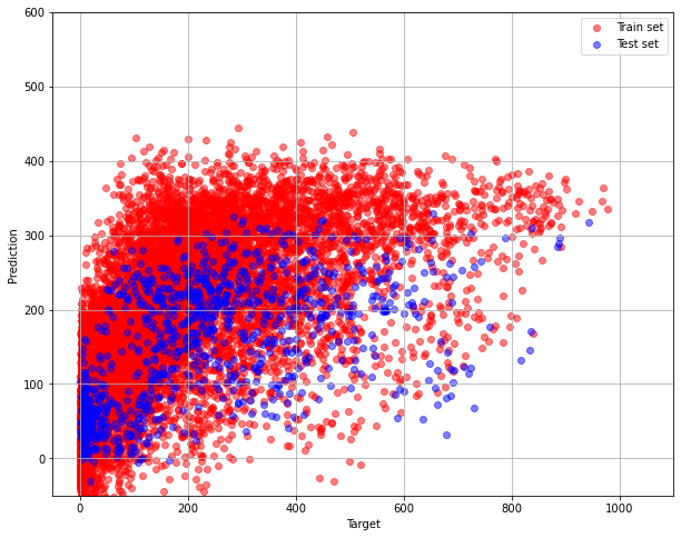
The graph is far from ideal, that is one with diagonal dependence. It resembles the Target-prediction graph from part 1.
Nonlinear model – Random Forest Regressor
We can make and use a different model, one that is more complex. The model that is able to take into account the nonlinear dependencies between the features and the target function.
from sklearn.ensemble import RandomForestRegressor
regressorRF = RandomForestRegressor(random_state = 0, max_depth = 20, n_estimators = 50)
estimator = pipeline.Pipeline(steps = [
("feature_processing", pipeline.FeatureUnion(transformer_list = [
	#binary
	("binary_variables_processing", preprocessing.FunctionTransformer(lambda data: data.iloc[:, binary_data_indices])),
	#numeric
	("numeric_variables_processing", pipeline.Pipeline(steps = [
		("selecting", preprocessing.FunctionTransformer(lambda data: data.iloc[:, numeric_data_indices])),
		("scaling", preprocessing.StandardScaler(with_mean = 0, with_std = 1))
				])),
	#categorical
	("categorical_variables_processing", pipeline.Pipeline(steps = [
		("selecting", preprocessing.FunctionTransformer(lambda data: data.iloc[:, categorical_data_indices])),
		("hot_encoding", preprocessing.OneHotEncoder(handle_unknown = "ignore"))
				])),
	])),
("model_fitting", regressorRF)
]
)
estimator.fit(train_data, train_labels)
Pipeline(steps=[("feature_processing",
 FeatureUnion(transformer_list=[("binary_variables_processing",
	 FunctionTransformer(func=<function <lambda> at 0x0000028328C430D0>)),
	("numeric_variables_processing",
	 Pipeline(steps=[("selecting",
		  FunctionTransformer(func=<function <lambda> at 0x0000028328C431F0>)),
		 ("scaling",
		  StandardScaler(with_mean=0,
						 with_std=1))])),
	("categorical_variables_processing",
	 Pipeline(steps=[("selecting",
		  FunctionTransformer(func=<function <lambda> at 0x0000028328C43CA0>)),
		 ("hot_encoding",
		  OneHotEncoder(handle_unknown="ignore"))]))])),
("model_fitting",
 RandomForestRegressor(max_depth=20,
 n_estimators=50, random_state=0))])
metrics.mean_absolute_error(test_labels, estimator.predict(test_data))
79.49758619912876
The MAE of RF model is less than one of SGD regressor model.
print("RF model\nLabel Prediction")
for l, p in zip(test_labels[:10], estimator.predict(test_data)[:10]):
    print( l, "   ", int(p))
RF model
Label Prediction
 525     409
 835     505
 355     256
 222     165
 228     205
 325     265
 328     254
 308     317
 346     280
 446     434
pylab.figure(figsize=(16, 6))
pylab.subplot(1,2,1)
pylab.grid(True)
pylab.xlim(-10,1100)
pylab.ylim(-10, 1000)
pylab.scatter(train_labels, grid_cv.best_estimator_.predict(train_data), alpha=0.5, color = "red", label = "Train set")
pylab.scatter(test_labels, grid_cv.best_estimator_.predict(test_data), alpha=0.5, color = "blue", label = "Test set")
pylab.title("Linear, SGD regressor model")
pylab.xlabel("Target")
pylab.ylabel("Prediction")
pylab.legend(loc="upper left")
pylab.subplot(1,2,2)
pylab.grid(True)
pylab.xlim(-10,1100)
pylab.ylim(-10,1000)
pylab.scatter(train_labels, estimator.predict(train_data), alpha=0.5, color = "red", label = "Train set")
pylab.scatter(test_labels, estimator.predict(test_data), alpha=0.5, color = "blue", label = "Test set")
pylab.title("Random Forest model")
pylab.xlabel("Target")
pylab.ylabel("Prediction")
pylab.legend(loc="upper left")
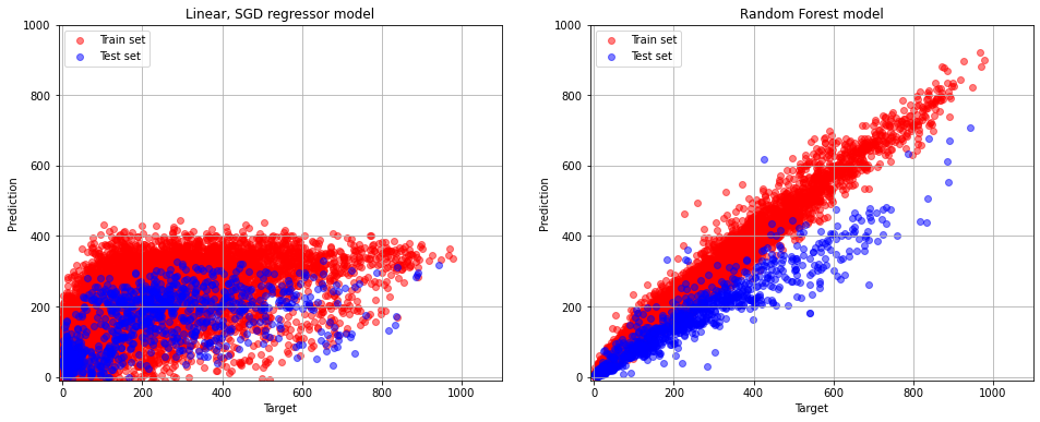
Compare SGD and RF model results
We see that in the case of RF the target-prediction objects are very close to the diagonal area. It turns out that with the RF model we managed to find much better dependency.