This short essay is about data mining methods applied in web traffic analysis and other business intelligence. It also provides a  modern look at data mining in light of the Big Data era.
For a site owner, business blogger or e-commerce entity, there are always some variables of interest concerning web traffic and statistics. How would you predict future values of variables of interest? Variables of interest might include the number of visitors to a target website, the time each visitor spends on the site, and whether or not the visitor reaches the site’s goals. One needs to mention that these web traffic and site performance analyses are not imposed with stringent time constraints. Data mining techniques seek to identify relationships between the variable of interest and the variables in a data sample. There are at least 3 analysis models for data mining that we consider here.

Analysis models

1. Predictive analysis: values for the variable of interest

Values for the variable of interest (e.g., the number of visitors to the website each month) are compared to the values for other variables in the dataset (e.g., the month of the year and the sum spent on advertising over the previous few months). The regression method would yield a fitted model, which is an equation that expresses the predicted number of monthly visitors as a linear combination of the other variables in the dataset (linear equations system), with weights determined by the regression analysis of the sample of data. This business intelligence predicts future site traffic and is able to assist in decisions such as whether to invoke additional marketing services or when to move to high speed servers.

An older but very usable tool, especially for an inexperienced user, is the DataMiningFox application which applies a prediction model to CSV data samples of almost any kind. When I tried it I  found it to be a worthwhile and handy non-professional data mining application. It can be used for Linux, Win and Mac. 

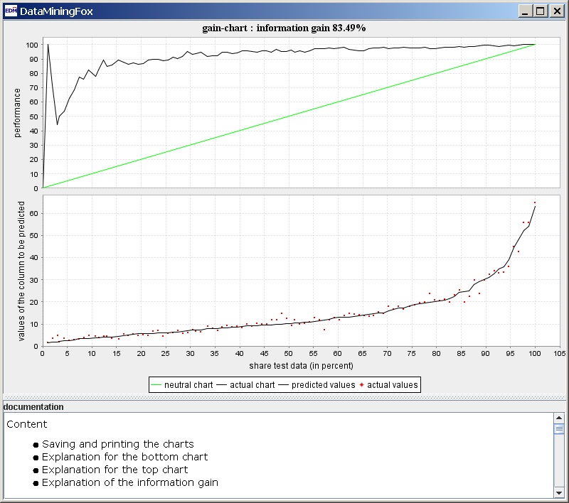
The upper graph black line indicates the performance, how close the values of the built model are to the original data samples. It yields better values as the data set increases.

I would mention that this tool builds both predictive and also classifying analysis models (see next paragraph).

2. Classification: classifying groups of interest

Classification is another field for which data mining is involved. An example might be the lending decisions faced by creditors. Banks or other lending institutions regularly collect data from loan applicants, on which they base their decision whether or not to extend credit. The goal is to classify applicants as either good or bad credit risks.
Data mining here would be used to identify relationships between the payment record and other variables in the data sample, relationships that would then form the basis of a “recipe” for classifying future applicants. The most common “recipe” is a decision tree. For visitors conversions, data mining establishes relationships between conversion rate and siteís pages visited, or average time spent, or some other variables. When the decision tree is formed, this “recipe” might be applied, with some error rate, to the new site visitors, analyzing their behavior as to prediction of conversions.

3. Associations: relationships among the variables (what goods are together in consumer basket?)

What are the interesting relationships among the variables we observe? The canonical example is the famous “shopping basket” question that asks which items tend to show up together in the purchases made by customers.
Another application as to the web traffic analysis is whether or not there are groups of pages that users tend to visit together? The presence of such groups can give a website owner valuable insight into how people use the site. For example, content split on separate pages but still often viewed together can be merged to achieve the smoothest and quickest browsing experience, and website pages which are visited only to reach other more important pages can be removed.

Overfit issue

These data mining techniques (not just decision trees) tend to overfit data. They fit given samples into a certain system (ex. linear equation system) for further application to future data sets. The systemís error rate is the main concern.

Error calculation

To calculate the error rate (ex. decision trees data mining) we take each loan application in the training set and use the model to classify it as either a good or bad credit risk. Then we check whether the actual outcome matches the classification assigned by our scheme. The ratio of errant classifications to the total number of applicants is the error rate for the training set.

Crucial notion: real error rate is likely to be much higher than the one calculated

The important point, however, is that the error rate is not a good indicator of the real error rate that we are likely to observe when we attempt to classify new loan applicants. In fact, the error rate for new applicants is likely to be higher, possibly significantly higher. The reason for this is that the structure of the decision tree we are using in this example is highly dependent on the training set itself. As the result, we apply the data mining with the inherent problem of overfitting. The reason – there is always an idiosyncrasy in the training set.

Modern statistical techniques

Partition model with large data sets

How about we divide the total data into two large sets, one for training and one for testing. This implies that we have large data sets. Techniques are done as previously, yet the error rate is calculated the same way as described above, except the observations in the test set are used instead of those in the training set. Since the tree was not created using the test set, performance on the test set is a reasonably accurate measure of performance on new data. New Error=Error(test set), not of training set.

Stricter approach with 3 data sets: Training, Validation and Test set. This uses more resources, but gives better accuracy. The data mining procedure is then expanded to three stages.

• First stage: several different algorithms are run on the training set.
• Each of these algorithms are then tested on a second dataset known as the validation set, at which time the best performing model is selected.
• Finally, the selected model is tested against a third set of data, the test set.

If data amount is not sufficient, a tradeoff must occur between the size of the training set and test set.

Holdout sampling

Repeated holdout sampling begins by randomly dividing the total dataset into a test and training set and proceeding as above. An error rate is determined based on performance over the test (“holdout”) set. This process is then repeated a number of times, and the resulting errors are averaged.

Cross-validation

The related technique of cross-validation randomly partitions the dataset into N subsets. Each of the subsets is used in turn as a test set, while the remaining sets are aggregated and used for training. This yields an error rate for each of the N subsets, and these N rates are then averaged to produce an overall error rate estimate. The number of partitions is arbitrary, ten being a popular choice.
Another technique to apply in data mining is a bootstrapping, which relies on the statistical procedure of sampling with replacement.

Conclusion

The cross-validation and bootstrapping techniques have been vital in modern data mining for applied analytics. Modern business intelligence with rapidly accumulated data might fully use these data mining techniques for given purposes. This allows businesses to confidently apply the knowledge derived from their accumulated data for succesful business intelligence.