The Regularization is applying a penalty to increasing the magnitude of parameter values in order to reduce overfitting. When you train a model such as a logistic regression model, you are choosing parameters that give you the best fit to the data. This means minimizing the error between what the model predicts for your dependent variable given your data compared to what your dependent variable actually is.

See the practical example how to deal with overfitting by the regularization.

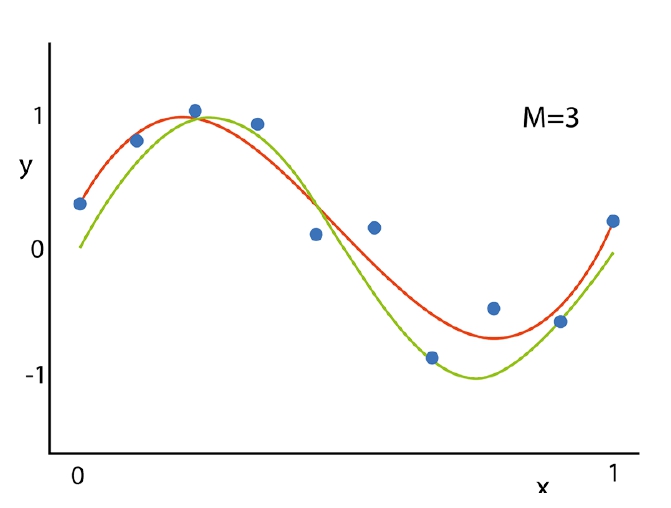
1. Normal model; the approximation function (red) of a trained model. It’s quite close to the true dependence (green),

y(x) = w₀ + w₁*x₁ + w₂*x₂ + w₃*x₃

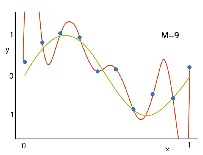
2. Overfitted model; its approximation function (red) fits ideal to the given train dataset (blue dots), yet fails to correctly predict future data.

y(x) = w₀ + w₁*x₁ + w₂*x₂ + … + w₉*x₉

3. The solution to that overfitting/overtraining would be adding a penalty to the MSE/MAE function thus issuing in regularization L. The latter we are to optimize.

L(w, x) = Q( w, x ) + λ|w| —> min(w)

• L1 (Lasso regression). The penalty is proportional to the sum of weights.
  
  .
• L2 (Ridge regression or Tikhonov regularization). The penalty is proportional to the sum of squared weights.
  
  .