
In this post we’ll share with you the vivid yet simple application of the Linear regression methods. We’ll be using the example of predicting a person’s height based on their weight. There you’ll see what kind of math is behind this. We will also introduce you to the basic Python libraries needed to work in the Data Analysis.
The iPython notebook code
Contents
1. The linear algebra and data processing libraries references
Seaborn is not included in the Anaconda build by default, but the library provides convenient high-level functionality for data visualization. To install it run the conda install seaborn command in the terminal.
2. Initial Data Analysis
We’ll be using the SOCR data on the weights and heights of 25’000 teenagers.
import numpy as np
import pandas as pd
import seaborn as sns
import matplotlib.pyplot as plt
%matplotlib inline
Load the data from weights_heights.csv file into a Pandas DataFrame, called data.
data = pd.read_csv('weights_heights.csv', index_col='Index')
data.head(5)
| Index | Height | Weight |
|---|---|---|
| 1 | 65.78331 | 112.9925 |
| 2 | 71.51521 | 136.4873 |
| 3 | 69.39874 | 153.0269 |
| 4 | 68.21660 | 142.3354 |
| 5 | 67.78781 | 144.2971 |
2.2 Primary Data Analysis
Let’s build histograms of the distribution of the features. This makes us to understand the nature of a feature (its distribution in particular). The histogram lets us to find such data values that stand out from the main data values, “outliers“. It is convenient to plot histograms using the plot Pandas DataFrame method with the kind argument=’hist’.
data.plot(y='Height', kind='hist',
color='g',  title='Height (inch.) distribution')
data.plot(y='Weight', kind='hist',
color='b',  title='Weight (pounds) distribution')


2.3 Adding the Body Mass Index, BMI
We add a third attribute, Body Mass Index BMI. Now the data are of more columns.
So, if we hitdata.head(5) we get the following result:
| Index | Height | Weight | BMI |
|---|---|---|---|
| 1 | 65.78331 | 112.9925 | 18.357573 |
| 2 | 71.51521 | 136.4873 | 18.762577 |
| 3 | 69.39874 | 153.0269 | 22.338895 |
| 4 | 68.21660 | 142.3354 | 21.504526 |
| 5 | 67.78781 | 144.2971 | 22.077581 |
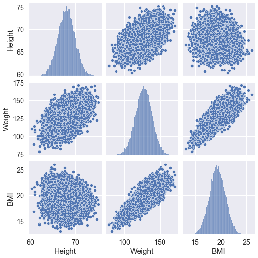
Now we display of pairwise dependencies of the features. Created 𝑚×𝑚 graphs (m is the number of features), where the diagonal cells depict histogram of the distribution of that feature and the rest of the cells show scatter plots based on two paired characteristics.
Let’s use the pairplot() method of the Seaborn library.
def make_bmi(height_inch, weight_pound):
    METER_TO_INCH, KILO_TO_POUND = 39.37, 2.20462
    return (weight_pound / KILO_TO_POUND) \       / (height_inch / METER_TO_INCH) ** 2

data['BMI'] = data.apply(lambda row: make_bmi(row['Height'],                                          row['Weight']), axis=1)
sns.set(font_scale=1.3)
sns.pairplot(data)
2.4 Adding a categorical feature
Let’s add a categorical feature, called weight_category. It takes only 3 values, [1,2,3], and is calculated as shown below.
def weight_category(weight):
    if weight < 120:
	    return 1
    elif weight >= 150:
	    return 3
    return 2
Box plot is a compact way to show statistics of a real feature (mean and quartiles) for different values of a categorical feature. It also helps to track “outliers“, the observations in which the value of this real feature is very different from others.
data['weight_cat'] = data['Weight'].apply(weight_category)
dataBoxplot = sns.boxplot(x='weight_cat', y='Height', data=data)
dataBoxplot.set(xlabel = 'Weight Category', ylabel = 'Height')
plt.show()

The problem of predicting the value of a real feature based on other features (the regression recovery problem) is solved by minimizing the quadratic error function.
3.1 Linear approximation function
We try to approximate dependence of the height on the weight by the following linear function: y(x) = w0 + w1*x
- y – height
- x – weight
- w0 и w1 are the scalar parameters, subject to the optimization.
3.2 Mean squared error (MSE) of the linear approximation function
The following function calculates squared error of the linear approximation y(x):
Error(w0, w1) = 1/n * ∑(yi – (w0 + w1 * xi))2
- n – number of observations in the data set.
- yi and xi – height and weight of i-th item in the data set.
Calculating and optimizing MSE, we’ll find the optimal w0 and w1 for the approximation. Below is the Python error function that calculates MSE based on the n samples of the data set.
def error(w0, w1, n):
    sum = 0
    for v in data.sample(n).values:
	    sum += (v[0] - (w0 + w1*v[1]))**2
    return np.round(sum/n)
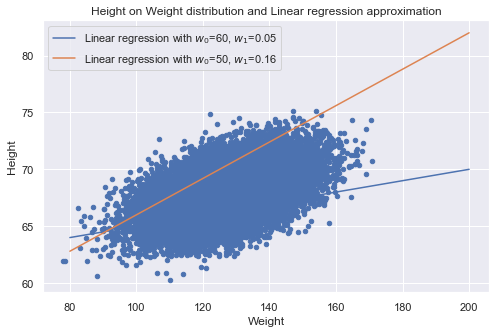
Now we plot both:
- (1) The cloud of points corresponding to the data set items as the space of the features height and weight.
- (2) Lines y(x) with approximate w0, w1. We’ll see if they convey the dependence of height on weight correctly.
# original data distribution
data.plot(x="Weight", y='Height', kind='scatter',
     color='b',  title='Height on Weight distribution and Linear regression approximation' )
plt.rcParams["font.size"] = "12"
# 100 samples (values) from 80 till 200
x = np.linspace(80, 200, 100)
plt.rcParams["figure.figsize"] = [8,5]
# Linear approximation parameters: sets of w0 and w1
sets = ([60, 0.05], [50, 0.16])
for s in sets:
    y = s[0] + s[1]*x
    plt.plot(x, y, label="Linear regression with w0={0}, w1={1}".format(*s))
plt.legend()
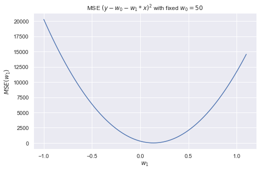
3.3 MSE graph
The MSE optimization is a relatively simple task, since the MSE is convex, namely y(x) ≈ x2. Later we leverage some optimization methods. Let’s see how the error function depends on one parameter only (the slope of the straight line, w1), if the second parameter (the free term, w0) is fixed.
x = np.linspace(-1, 1.1, 110)
plt.rcParams["figure.figsize"] = [8,5]
plt.rcParams["font.size"] = "15"
plt.plot(x, error(50, x, 10))
plt.title('MSE (y - w0 - w1*x)^2 with fixed w0=50')
plt.ylabel('MSE(w1)')
plt.xlabel('w1')
3.4 MSE optimization with one fixed parameter
Now, we optimize to find an optimal line slope (w1), approximating height on weight dependency with fixed w0 = 50.
We use minimize_scalar method from scipy.optimize for MSE where w1 ∈ [-5,5].
def err_f(x):
    return error(50, x, 100)
from scipy.optimize import minimize_scalar
w1 = minimize_scalar(err_f, bounds = (-5, 5), method='bounded')
print('Min MSE with w1 =', w1.x)
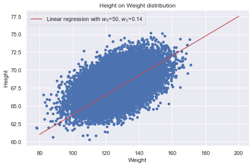
Min MSE with w1 = 0.13747647556112128
Let’s plot the height on weight distribution along with the linear approximation using the optimized parameter w1.
data.plot(x="Weight", y='Height', kind='scatter',       color='b',  title='Height on Weight distribution' )
x = np.linspace(80, 200, 100)
y = 50 + w1.x*x
plt.plot(x, y, label="Linear regression with w0=50, w1=0.14", color='r')
plt.legend()
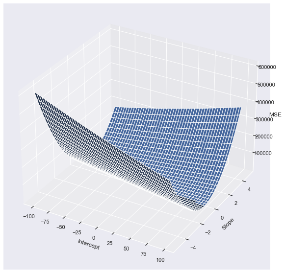
3.5 Plot MSE as 3-D grid
We now plot the MSE 3D-grids with parameters w0 and w1.
- Axis X is «Intercept»
- Axis Y is «Slope»
- Axis Z is «MSE»
We use numpy.meshgrid that return coordinate matrices from coordinate vectors.
We create objects of type matplotlib.figure.Figure (figure) and matplotlib.axes._subplots.Axes3DSubplot (axis).
from mpl_toolkits.mplot3d import Axes3D
fig = plt.figure()
fig.set_size_inches(20,10)
ax = fig.gca(projection='3d') # get current axis
w0 = np.arange(-100, 100, 1)
w1 = np.arange(-5, 5, 0.25)
X, Y = np.meshgrid(w0, w1)
Z = error(X, Y, 10)

# Method `plot_surface` of Axes3DSubplot
surf = ax.plot_surface(X, Y, Z)
ax.set_xlabel('Intercept')
ax.set_ylabel('Slope')
ax.set_zlabel('MSE')
plt.show()
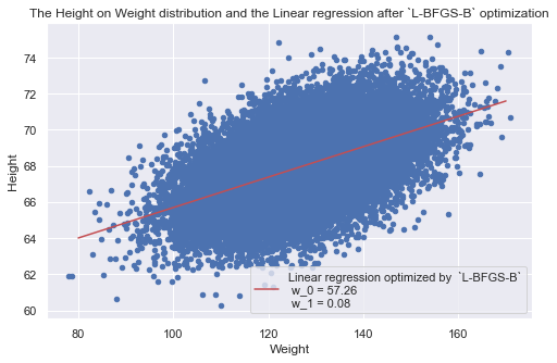
3.6 MSE optimization using the L-BFGS-B method
We use minimize of the scipy.optimize library to minimize MSE from point 3.2.
- w0 ∈ [-100,100] and w1 ∈ [-5, 5].
- initial guess point (w0, w1) = (0, 0).
We use the L-BFGS-B method and later we plot the height on weight distribution along with the Linear approximation for optimized w0 and w1.
import scipy.optimize as optimize
def error1(w):
    s = 0
    x = data['Weight']
    y = data['Height']
    for i in range(1, int(len(data.index)/100)):
	    s = s + (y[i] - w[0] - w[1] * x[i]) ** 2
    return s
optimum = optimize.minimize(error1, np.array([0,0]), method = 'L-BFGS-B', bounds = ((-100, 100), (-5, 5)))
print(optimum)
fun: 667.5124003407069


  hess_inv: <2x2 LbfgsInvHessProduct with dtype=float64>


  jac: array([0.00010232, 0.02563638])


  message: b'CONVERGENCE: REL_REDUCTION_OF_F_<=_FACTR*EPSMCH'


  nfev: 54


  nit: 7


njev: 18


  status: 0


  success: True


  x: array([57.26076187,  0.08431683])
data.plot(x="Weight", y='Height', kind='scatter',
        color='b',  title='The Height on Weight distribution and the Linear regression after `L-BFGS-B` optimization' )
x = np.linspace(80, 170, 100)
y = optimum.x[0] + optimum.x[1]*x
plt.plot(x, y, label="Linear regression optimized by  `L-BFGS-B`" \    +"\n w0 = {0}\n w1 = {1}".format(np.round(optimum.x[0], 2), np.round(optimum.x[1], 2)), color="r")
plt.legend()
4. Conclusion
In this post we’ve applied the Linear regression approximation to the given data set. Then we’ve used the MSE as the means for optimizing the linear regression approximation function. Using the linear algebra methods we could successfully find optimal parameters for the linear regression approximation function.