import pandas as pd
import numpy as np
from matplotlib import pyplot as plt
%matplotlib inline

df = pd.read_csv("bikes_rent.csv")
df.head()

   season  yr  mnth  holiday  weekday  workingday  weathersit
0       1   0     1        0        6           0           2
1       1   0     1        0        0           0           2
2       1   0     1        0        1           1           1
3       1   0     1        0        2           1           1
4       1   0     1        0        3           1           1
        temp     atemp      hum  windspeed(mph)  windspeed(ms)   cnt
0  14.110847  18.18125  80.5833       10.749882       4.805490   985
1  14.902598  17.68695  69.6087       16.652113       7.443949   801
2   8.050924   9.47025  43.7273       16.636703       7.437060  1349
3   8.200000  10.60610  59.0435       10.739832       4.800998  1562
4   9.305237  11.46350  43.6957       12.522300       5.597810  1600

For each rental day, the following attributes/dataset features are known (as they were specified in the data source):

• season: 1-spring, 2-summer, 3-autumn, 4-winter
• yr: 0 – 2011, 1 – 2012
• mnth: from 1 to 12
• holiday: 0 – no holiday, 1 – there is a holiday
• weekday: 0 to 6
• workingday: 0 – non-working day, 1 – working day
• weathersit: weather favorability rating from 1 (clear day) to 4 (rain, fog)
• temp: temperature in Celsius degrees
• atemp: temperature feels like, Celsius degrees
• hum: humidity
• windspeed(mph): wind speed in miles per hour
• windspeed (ms): wind speed in meters per second
• cnt: the number of rented bicycles (this is the target attribute, we will predict it thru a built model)

So, we have real (temp atemp, hum, windspeed(mph), windspeed(ms)), binary (holiday, workingday), and nominal (ordinal) features (eg. season: 1-spring, 2-summer, 3-autumn, 4-winter; weekday, weathersit). All of them might be worked with as real features.

One can work with nominal attributes as with real ones, because they are in an order. Let’s look at the figures below, showing how the target attribute (cnt) depends on each of the features.

Feature target plots

fig, axes = plt.subplots(nrows=3, ncols=4, figsize=(15, 10))
for idx, feature in enumerate(df.columns[:-1]):
    df.plot(feature, "cnt", subplots=True,  kind="scatter", ax=axes[idx // 4, idx % 4])

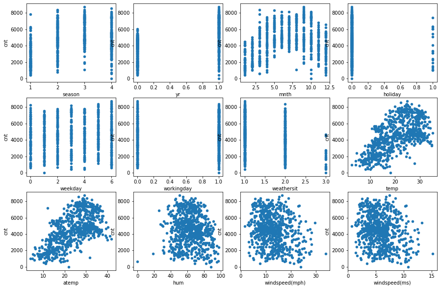
One can see from the charts that there is the linear dependence of the target of some features, eg. season, atemp.

Features and target correlations

Pairwise correlations between all featues except for the target

Let’s more strictly estimate the level of linear dependence between the features and the target variable. A good measure of the linear relationship between two vectors is the Pearson correlation. In the Pandas it can be calculated using two dataframe methods: corr and corrwith. The df.corr method calculates the correlation matrix of all features from the dataframe. The df.corrwith method needs to supply another dataframe as an argument, and then it will calculate pairwise correlations between the features from the function argument and the original dataframe.

# df2 - df without the column "cnt", the target
df2 = df[df.columns[:-1]]
# alternative: df2 = df[df.columns.difference(["cnt"])]
# get features correlation coefficients
df2.corr(method="pearson")

                      season         yr       mnth        holiday      weekday    workingday    weathersit    temp        atemp       hum       windspd(mph) windspd(ms)
season              1.000000    -0.001844    0.831440    -0.010537    -0.003080    0.012485    0.019211     0.334315    0.342876    0.205445     -0.229046    -0.229046
yr                 -0.001844    1.000000    -0.001792    0.007954    -0.005461    -0.002013    -0.048727    0.047604    0.046106    -0.110651    -0.011817    -0.011817
mnth               0.831440    -0.001792    1.000000     0.019191    0.009509    -0.005901    0.043528      0.220205    0.227459    0.222204     -0.207502    -0.207502
holiday            -0.010537    0.007954    0.019191     1.000000    -0.101960    -0.253023    -0.034627    -0.028556   -0.032507    -0.015937    0.006292    0.006292
weekday            -0.003080    -0.005461    0.009509    -0.101960    1.000000    0.035790    0.031087      -0.000170   -0.007537    -0.052232    0.014282    0.014282
workingday         0.012485    -0.002013    -0.005901    -0.253023    0.035790    1.000000    0.061200      0.052660    0.052182    0.024327     -0.018796    -0.018796
weathersit         0.019211    -0.048727    0.043528     -0.034627    0.031087    0.061200    1.000000      -0.120602   -0.121583    0.591045    0.039511    0.039511
temp               0.334315    0.047604     0.220205     -0.028556    -0.000170    0.052660    -0.120602    1.000000    0.991702    0.126963     -0.157944    -0.157944
atemp              0.342876    0.046106     0.227459     -0.032507    -0.007537    0.052182    -0.121583    0.991702    1.000000    0.139988     -0.183643    -0.183643
hum                0.205445    -0.110651    0.222204     -0.015937    -0.052232    0.024327    0.591045    0.126963     0.139988    1.000000     -0.248489    -0.248489
windspeed(mph)     -0.229046    -0.011817    -0.207502    0.006292    0.014282    -0.018796    0.039511    -0.157944    -0.183643    -0.248489    1.000000    1.000000
windspeed(ms)      -0.229046    -0.011817    -0.207502    0.006292    0.014282    -0.018796    0.039511    -0.157944    -0.183643    -0.248489    1.000000    1.000000

# kitchen sink solution: pd.concat([df,df],axis=1).corr()
df.corrwith(df["cnt"], axis=0, method="pearson")

season            0.406100
yr                0.566710
mnth              0.279977
holiday          -0.068348
weekday           0.067443
workingday        0.061156
weathersit       -0.297391
temp              0.627494
atemp             0.631066
hum              -0.100659
windspeed(mph)   -0.234545
windspeed(ms)    -0.234545
cnt               1.000000
dtype: float64

The sample above shows features correlations with the target. All of them are not null. That means that we can solve the problem using linear methods.

The graphs above show that some of the features are similar to each other. So let’s also calculate the correlations between the real features: temp, atemp, hum, windspeed(mph), windspeed(ms) and cnt

df3 = df[["temp", "atemp", "hum", "windspeed(mph)", "windspeed(ms)", "cnt"]]
df3.corr(method="pearson")

                  temp       atemp       hum     windspeed(mph)    windspeed(ms)     cnt
temp               1.000000    0.991702    0.126963    -0.157944        -0.157944        0.627494
atemp              0.991702    1.000000    0.139988    -0.183643        -0.183643        0.631066
hum                0.126963    0.139988    1.000000    -0.248489        -0.248489        -0.100659
windspd(mph)      -0.157944    -0.183643   -0.248489    1.000000        1.000000         -0.234545
windspeed(ms)     -0.157944    -0.183643   -0.248489    1.000000        1.000000         -0.234545
cnt                0.627494    0.631066    -0.100659    -0.234545        -0.234545        1.000000

As expected, there are ones 1 on the diagonals. However, there are two more pairs of strongly correlated columns in the matrix: temp and atemp (correlated by nature) and two windspeed features (because one is just a translation of some units into others). Later we will see that this effects negatively on the training of the linear model.

Let’s take a look at the mean values of the features to estimate the scale of the features and the fraction of 1 for binary features.

df.mean()

season               2.496580
yr                   0.500684
mnth                 6.519836
holiday              0.028728
weekday              2.997264
workingday           0.683995
weathersit           1.395349
temp                20.310776
atemp               23.717699
hum                 62.789406
windspeed(mph)      12.762576
windspeed(ms)        5.705220
cnt               4504.348837
dtype: float64

The features are of different scale. So for our further work, we better normalize the feature objects matrix.

Problem one: Collinear (highly correlated) features

So, in our data, some attributes duplicates another ones and there are two more very similar ones. Of course, we could remove the duplicates right away, but let’s see how model would have been trained if we hadn’t noticed this problem.

To begin with, we will scale or standardize the features. From each feature, we will subtract its average (mean) and divide it by the standard deviation (std). This can be done using the scale() method.

In addition we shuffle the dataset; this is required for cross-validation.

from sklearn.preprocessing import scale
from sklearn.utils import shuffle

df_shuffled = shuffle(df, random_state=123)
print(df_shuffled.head())
X = scale(df_shuffled[df_shuffled.columns[:-1]])
y = df_shuffled["cnt"]

     season  yr  mnth  holiday  weekday  workingday  weathersit       temp  \
488       2   1     5        0        4           1           2  22.960000   
421       1   1     2        0        0           0           1  11.445847   
91        2   0     4        0        6           0           2  12.915000   
300       4   0    10        0        5           1           2  13.564153   
177       3   0     6        0        1           1           2  27.982500   
        atemp      hum  windspeed(mph)  windspeed(ms)   cnt  
488  26.86210  76.8333        8.957632       4.004306  6421  
421  13.41540  41.0000       13.750343       6.146778  3389  
91   15.78185  65.3750       13.208782       5.904686  2252  
300  15.94060  58.5833       15.375093       6.873086  3747  
177  31.85020  65.8333        7.208396       3.222350  4708  

Train linear model

Let’s train a linear regression model on our dataset and look at the feature weights. The acquired weights are in the coef_ parameter of a regressor class.

from sklearn.linear_model import LinearRegression

from sklearn import linear_model
  # build a model
linear_regressor = linear_model.LinearRegression() 
  # train the model using all data
linear_regressor.fit(X, y)  
  # output coefficients
print("Linear model coefficients:\n", linear_regressor.coef_ )
    # get the model predictions 
    # predictions = linear_regressor.predict() 
print("\nCoefficients and their weights:")
[(pair[0], round(pair[1],2)) for pair in zip(df.columns, linear_regressor.coef_)]

Linear model coefficients:
 [ 5.70865954e+02  1.02196587e+03 -1.41301029e+02 -8.67565864e+01
  1.37223034e+02  5.63936928e+01 -3.30228163e+02  3.67479222e+02
  5.85554695e+02 -1.45612324e+02  1.24575770e+13 -1.24575770e+13]

Coefficients and their weights:
 [("season", 570.87),
 ("yr", 1021.97),
 ("mnth", -141.3),
 ("holiday", -86.76),
 ("weekday", 137.22),
 ("workingday", 56.39),
 ("weathersit", -330.23),
 ("temp", 367.48),
 ("atemp", 585.55),
 ("hum", -145.61),
 ("windspeed(mph)", 12457576985764.57),
 ("windspeed(ms)", -12457576985963.02)]

We see that the weights for linearly dependent features are significantly greater in absolute values than for other features.

To better understand why this happened, let’s recall the analytical formula used to calculate the weights of a linear model in the least squares method:

w = (X^TX)^-1* X^T* y

If there are collinear (linearly dependent) columns in X, the matrix X^TX becomes degenerate one. The formula then ceases to be correct. The more dependent the features are, the smaller the determinant of this matrix is and the worse the approximation of 𝑋*𝑤≈𝑦 is. This situation is called the multicollinearity problem.

The temp-atemp pair had slightly less correlated variables/weights. But in practice, one should always carefully monitor the coefficients for similar attributes.

The multicollinearity problem solution is to regularize the linear model. The norm of weights multiplied by the regularization coefficient alpha, α, (L1 or L2), is added to the optimized functional X*w. In the first case (L1), the method is called Lasso, and in the second (L2), the method is called Ridge. Read more about the adding regularization into a Linear Regression model.

We train the Ridge и Lasso regressors with the default parameters and make sure that the problem with the weights is resolved.

from sklearn.linear_model import Lasso, Ridge
lasso = Lasso()
lasso.fit(X, y)
print("Lasso regularization coefficients/weights:\n", lasso.coef_)
print("\nIntercept:", lasso.intercept_)
print( "\nRounded coef:", list(map(lambda c: round(c, 3) , lasso.coef_) )) 

Lasso regularization coefficients/weights:
 [ 5.60241616e+02  1.01946349e+03 -1.28730627e+02 -8.61527813e+01
  1.37347894e+02  5.52123706e+01 -3.32369857e+02  3.76363236e+02
  5.76530794e+02 -1.44129155e+02 -1.97139689e+02 -2.80504168e-08]
Intercept: 4504.3488372093025
Rounded coef: [560.242, 1019.463, -128.731, -86.153, 137.348, 55.212, 
-332.37, 376.363, 576.531, -144.129, -197.14, -0.0]

ridge = Ridge()
ridge.fit(X, y)
print("Ridge regularization coefficients/weights:\n", ridge.coef_)
print("\nIntercept:", ridge.intercept_)
print("\nRounded coef:", list(map(lambda c: round(c, 3) , ridge.coef_) )) 

Ridge regularization coefficients/weights:
 [ 563.06457225 1018.94837879 -131.87332028  -86.746098    138.00511118
   55.90311038 -332.3497885   386.45788919  566.34704706 -145.0713273
  -99.25944108  -99.25944115]
Intercept: 4504.3488372093025
Rounded coef: [563.065, 1018.948, -131.873, -86.746, 138.005, 55.903, -332.35, 386.458, 566.347, -145.071, -99.259, -99.259]

Problem two: Uninformative features

In contrast to L2 regularization, L1 resets the weights for some features.

Model coefficients as function of alpha

Let’s see how the weights change with an increase in the regularization coefficient alpha.

coefs_lasso is the matrix of weights of size: (number of regressors) x (number of features).

alphas = np.arange(1, 500, 50)
coefs_lasso = np.zeros((alphas.shape[0], X.shape[1])) 

For each coefficient value from alphas set we train the Lasso regressor and write the weights into the corresponding rows of the coefs_lasso matrix. Then we train the Ridge regressor and write the weights into coefs_ridge matrix.

print("Matrix `coefs_lasso` size:", (alphas.shape[0], X.shape[1]), "\nAlpha values:", alphas )
for i, al in enumerate(alphas):
    lasso = Lasso(alpha = al)
    lasso.fit(X, y)
    for j, coef in enumerate(lasso.coef_):
        coefs_lasso[i][j]=coef
    #print(list(map(lambda c: round(c, 3) , coefs_lasso[i]) ))
# list(map(lambda c: round(c, 3) , coefs_lasso) ))
print("Lasso coefficients, head:\n", coefs_lasso[:5])
print("\nRounded Lasso coefficients:\n", list(map(lambda i: list(map(lambda j: round(j, 3), i)), coefs_lasso)))

Matrix `coefs_lasso` size: (10, 12) 
  
Alpha values: [  1  51 101 151 201 251 301 351 401 451]

Lasso coefficients, head:
 [[ 5.60241616e+02  1.01946349e+03 -1.28730627e+02 -8.61527813e+01
   1.37347894e+02  5.52123706e+01 -3.32369857e+02  3.76363236e+02
   5.76530794e+02 -1.44129155e+02 -1.97139689e+02 -2.80504168e-08]
 [ 4.10969632e+02  9.77019409e+02 -0.00000000e+00 -5.34489688e+01
   9.19434374e+01  1.75372118e+01 -3.18125568e+02  3.22829934e+02
   6.10031512e+02 -9.10689615e+01 -1.45066095e+02 -2.29877063e-08]
 [ 3.70077089e+02  9.35945490e+02  0.00000000e+00 -1.21619360e+01
   4.88886342e+01  0.00000000e+00 -3.08805664e+02  2.69417263e+02
   6.32502623e+02 -2.75042876e+01 -9.37749037e+01 -2.41652170e-08]
 [ 3.32835717e+02  8.91870058e+02  0.00000000e+00 -0.00000000e+00
   0.00000000e+00  0.00000000e+00 -2.79616688e+02  2.11052030e+02
   6.62920880e+02 -0.00000000e+00 -5.01551472e+01 -2.62761604e-08]
 [ 2.98134448e+02  8.45652857e+02  0.00000000e+00 -0.00000000e+00
   0.00000000e+00  0.00000000e+00 -2.35571345e+02  1.24144807e+02
   7.25379483e+02 -0.00000000e+00 -1.26461769e+01 -2.78781252e-08]]
   
Rounded Lasso coefficients:
 [[560.242, 1019.463, -128.731, -86.153, 137.348, 55.212, -332.37, 376.363, 576.531, -144.129, -197.14, -0.0], \
 [410.97, 977.019, -0.0, -53.449, 91.943, 17.537, -318.126, 322.83, 610.032, -91.069, -145.066, -0.0], \
 [370.077, 935.945, 0.0, -12.162, 48.889, 0.0, -308.806, 269.417, 632.503, -27.504, -93.775, -0.0], \
 [332.836, 891.87, 0.0, -0.0, 0.0, 0.0, -279.617, 211.052, 662.921, -0.0, -50.155, -0.0], \
 [298.134, 845.653, 0.0, -0.0, 0.0, 0.0, -235.571, 124.145, 725.379, -0.0, -12.646, -0.0], \
 [258.927, 799.237, 0.0, -0.0, 0.0, 0.0, -190.822, 72.076, 750.363, -0.0, -0.0, -0.0], \
 [217.428, 752.721, 0.0, -0.0, 0.0, 0.0, -145.713, 37.715, 756.297, -0.0, -0.0, -0.0], \
 [175.93, 706.204, 0.0, -0.0, 0.0, 0.0, -100.605, 3.661, 761.926, -0.0, -0.0, -0.0], \
 [134.628, 659.633, 0.0, -0.0, 0.0, 0.0, -55.511, 0.0, 737.348, -0.0, -0.0, -0.0], \
 [93.352, 613.055, 0.0, -0.0, 0.0, 0.0, -10.419, 0.0, 709.131, -0.0, -0.0, -0.0]]

coefs_ridge = np.zeros((alphas.shape[0], X.shape[1]))
for i, al in enumerate(alphas):
    ridge = Ridge(alpha = al)
    ridge.fit(X, y)
    for j, coef in enumerate(ridge.coef_):
        coefs_ridge[i][j]=coef
    print(list(map(lambda c: round(c, 3) , coefs_ridge[i]) ))

[563.065, 1018.948, -131.873, -86.746, 138.005, 55.903, -332.35, 386.458, 566.347, -145.071, -99.259, -99.259]
[461.179, 954.308, -41.565, -84.913, 126.604, 54.252, -313.275, 458.901, 481.444, -151.291, -101.627, -101.627]
[403.977, 898.084, 5.674, -81.911, 117.941, 52.728, -298.409, 455.29, 467.431, -152.686, -102.102, -102.102]
[366.604, 848.463, 34.027, -78.772, 110.68, 51.257, -286.125, 447.48, 455.754, -151.483, -102.005, -102.005]
[339.745, 804.251, 52.49, -75.717, 104.403, 49.842, -275.486, 438.51, 444.764, -148.944, -101.586, -101.586]
[319.159, 764.561, 65.152, -72.82, 98.879, 48.485, -266.003, 429.214, 434.235, -145.698, -100.965, -100.965]
[302.636, 728.709, 74.138, -70.099, 93.956, 47.185, -257.391, 419.926, 424.122, -142.089, -100.209, -100.209]
[288.913, 696.146, 80.66, -67.555, 89.529, 45.943, -249.471, 410.8, 414.409, -138.317, -99.361, -99.361]
[277.213, 666.43, 85.459, -65.179, 85.519, 44.757, -242.124, 401.912, 405.086, -134.499, -98.449, -98.449]
[267.031, 639.195, 89.012, -62.959, 81.865, 43.625, -235.264, 393.298, 396.138, -130.71, -97.493, -97.493]

The weights dependence on alpha dynamic

We visualize the dynamics of the weights as the regularization parameter alpha increases.

plt.figure(figsize=(10, 8))
for coef, feature in zip(coefs_lasso.T, df.columns):
    plt.plot(alphas, coef, label=feature, color=np.random.rand(3))
plt.legend(loc="upper right", bbox_to_anchor=(1.4, 0.95))
plt.xlabel("Alpha")
plt.ylabel("Feature weight")
plt.title("Lasso")
plt.figure(figsize=(10, 8))
for coef, feature in zip(coefs_ridge.T, df.columns):
    plt.plot(alphas, coef, label=feature, color=np.random.rand(3))
plt.legend(loc="upper right", bbox_to_anchor=(1.4, 0.95))
plt.xlabel("Alpha")
plt.ylabel("Feature weight")
plt.title("Ridge")

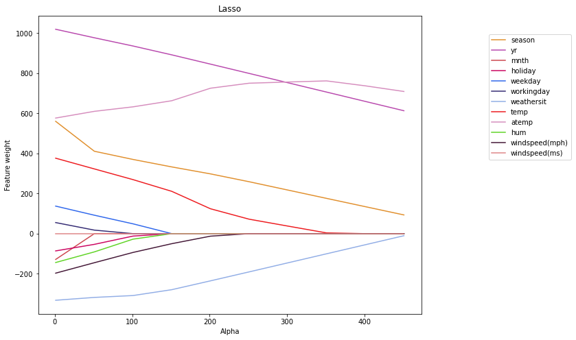
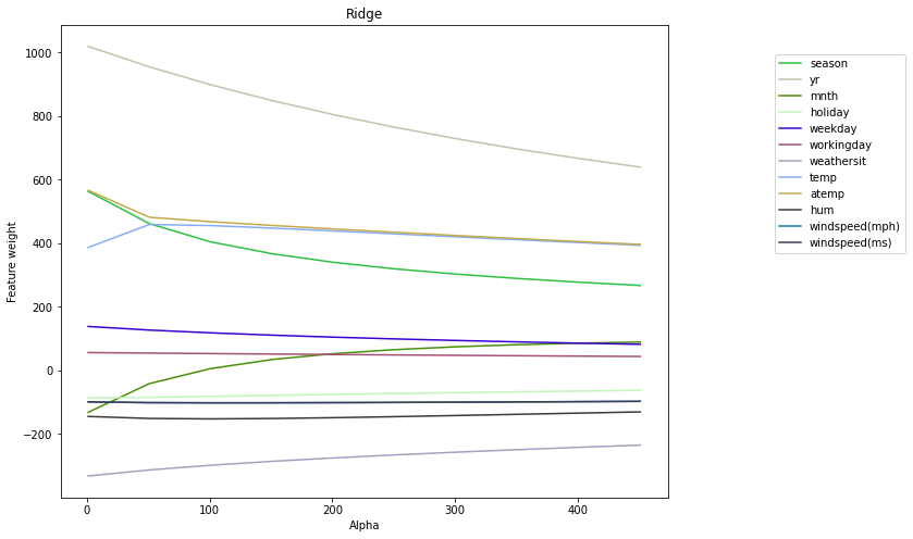
Sub-conclusions on Lasso and Ridge regularizators

We may do the following conclusions of the above figures:

1. Lasso regularizator reduces weights more aggressively than Ridge at the same alpha.
2. The regression model weights with the Lasso regularizator will tend/pursure to zero. The higher the alpha, the lower the complexity of the model. Then, for very large values of alpha, it is optimal to simply bring all the weights to zero.
3. It is assumed that the regularizator excludes a feature if the feature coefficient is less than 0.001 (<1e-3). At Lasso regularizator with alpha = 1, the weights for both “windspeeds” are not zero. But for alpha >= 50, the weights for both “windspeeds” are greatly reduced. As for the Ridge (L2) regularizator, the weights for collinear features depend little on alpha. Ridge does not exclude features when alpha increasing.
4. Lasso always excludes one of the duplicate attributes/features while Ridge only reduces the weight with one of them.
5. Lasso regularizator is more fitting for selecting uninformative features.

We will work with Lasso (L1) regularizator to optimize regression model with regularization

We might see that when alpha changes, the model selects the feature coefficients differently. We need to choose the best alpha then.

We first choose a quality metric. We will take the optimized functional of the least squares method, i.e. Mean Square Error (MSE), as a metric. Now, how to calculate MSE for different alpha?

Cross-validation

• We can’t choose alpha by the MSE value on the whole training sample
• We neither can choose a single split of the sample into training and test sets (“holdout”), since we will tune the model in to specific “new” data, namely the test set.
• The best approach is cross-validation. We divide the sample into K parts, or blocks, and each time take one of them as a test, and make a training sample from the remaining blocks. We will make several partitions of the sample, try different alpha values on each one, and then average the MSE.

The cross-validation for regression in sklearn library is quite simple: there is a special regressor for this, namely LassoCV. It takes as input a list of alphas and calculates the MSE for each of them on cross-validation. After training (parameter cv=3), the regressor will contain the variable mse_path_, a matrix of size len(alpha) x K, where K = 3 (the number of blocks in cross-validation), containing the MSE values on the test for the corresponding runs. In addition, the variable alpha_ will store the selected (optimal) value of the regularization parameter, and in coef_, will have the trained weights corresponding to this alpha_.

Note that the regressor can change the order in which it iterates through the alphas values. In order to map it to the MSE matrix, it is better to use the regressor variable alphas_.

from sklearn.linear_model import LassoCV

alphas = np.arange(1, 100, 5)
reg = LassoCV(cv=3, random_state=0, alphas = alphas )
reg.fit(X, y)
print("Regularizator score (coefficient of determination\n R^2 of the prediction):", reg.score(X, y))
print("\nRegularizator MSE matrix head:\n", reg.mse_path_[:5])
print("\nRegularizator\"s `Alpha`:", reg.alpha_)
print("\nRegularizator coefficients:")  
[(pair[0], round(pair[1], 4)) for pair in zip(df.columns[:-1], reg.coef_)]

Regularizator score (coefficient of determination
 R^2 of the prediction): 0.800081404381094
  
Regularizator MSE matrix head:
 [[863936.50981215 826364.11936907 862993.29751897]
 [860479.31511364 821110.1817776  853075.13780626]
 [857344.83606082 816153.27782428 843628.81286099]
 [854526.73639431 811496.34805693 834654.45357263]
 [852024.62341384 807139.39657173 826152.16399016]]
 
Regularizator`s `Alpha`: 6

Regularizator coefficients:
[("season", 532.019),
 ("yr", 1015.0602),
 ("mnth", -100.0395),
 ("holiday", -83.294),
 ("weekday", 132.5045),
 ("workingday", 51.5571),
 ("weathersit", -330.5599),
 ("temp", 370.6799),
 ("atemp", 581.3969),
 ("hum", -140.0074),
 ("windspeed(mph)", -191.7714),
 ("windspeed(ms)", -0.0)]

Plotting the mean MSE as a function of alpha.

mean_mse_arr = np.array(reg.mse_path_).mean(axis=1)
#print(mean_mse_arr)
plt.figure(figsize=(10, 8)) 
plt.plot(reg.alphas_, mean_mse_arr, label=feature ) 
plt.xlabel("Alpha")
plt.ylabel("Mean MSE by fold")
plt.title("Lasso regularizator MSE")

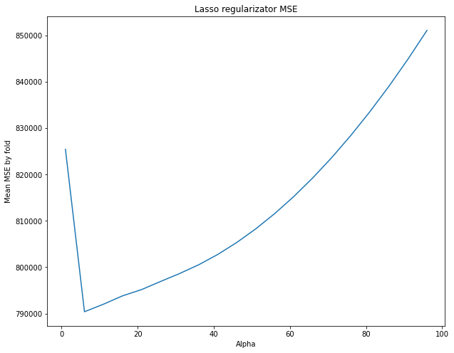
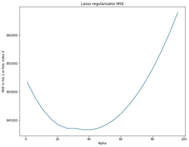
We have chosen a certain regularization parameter (alpha). Let’s look at what kind of alpha we would choose if we divided the dataset only once into training and test sets. We’ll consider the MSE graphs corresponding to single blocks (fold) of the dataset.

mse_columns = np.array(reg.mse_path_).transpose()
print("Minimum MSE for each column:", np.amin(mse_columns, axis=1), "\n" )
#print (reg.mse_path_)#[NumberOfColum])
for i, column in enumerate(mse_columns):
    print("MSE for column {}:".format(i) ,  column.mean() )
plt.figure(figsize=(10, 8)) 
plt.plot(reg.alphas_, mse_columns[0], label=feature ) 
plt.xlabel("Alpha")
plt.ylabel("MSE in the 1-st fold, index 0")
plt.title("Lasso regularizator MSE")

Minimum MSE for each column: [843336.18149882 772598.49562777 745668.60596081] 
MSE for column 0: 848818.027469035
MSE for column 1: 797903.087624002
MSE for column 2: 794699.8496187156

fig, axs = plt.subplots(len(mse_columns))
fig.set_size_inches(12,12)
fig.suptitle("MSE in each of 3 Folds")
for i, col in enumerate(mse_columns):
    axs[i].plot(reg.alphas_, col) 
    axs[i].set_xlabel("Alpha")
    axs[i].set_ylabel("MSE, fold {}".format(i))

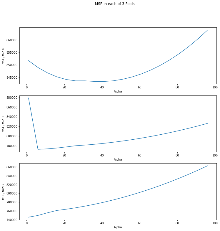
On each partition (fold), the optimal value of alpha is different. It might correspond to a large MSE on the other partitions. It turns out that we are tuning regularization parameter alpha in to specific training and control sets. When choosing alpha on cross-validation, we choose something “average” that will give an acceptable metric value on different dataset partitions.

Sub-conclusion on the Lasso regularization

1. In the last trained model, there are 4 features with the highest (positive) coefficients: ‘season’, ‘yr’, ‘temp’, ‘atemp’.
2. We may look at the visualizations of the `cnt` dependencies on these features that we drew in the “Dataset” block. There we may see increasing linear dependence of cnt on these features. It is logical to say (from common sense) that the greater the value of these feature weights, the more people will want to take bicycles.
3. We select the features with the largest modulo negative coefficients: ‘weathersit’, ‘ windspeed(mph)’, ‘hum’.
4. The graphs show a decreasing linear relationship with the target, cnt. It is logical to say that the greater the magnitude of these feature weights, the fewer people will want to take bicycles.
5. The feature windspeed (ms) has coefficient close to zero (less than 1e-3). The linear model excluded it since it is a correlated (collinear) feature with windspeed(mph) from the model. One may see it at the graphs there. It is true that this feature does not affect the demand for bicycles since windspeed (ms) has already influenced it.

Conclusion

In the post we’ve built a linear model and evaluated the adequacy of the model. We’ve learned how to select features, and how to correctly select the regularization coefficient alpha (without tuning in the model to any particular piece of data).

When using the cross-validation we selected only a small number of folds/partitions (3). It’s because for each valid combination of them, we have to train the model several times (for different alpha) that is a time-consuming process esp. for large amounts of data.