
in the post will reviewed a number of metrics for evaluating classification and regression models. For that we use the functions we use of the sklearn library. We’ll learn how to generate model data and how to train linear models and evaluate their quality.
The code as an IPython notebook
sklearn.metrics
import warnings
warnings.filterwarnings("ignore")
from sklearn import model_selection, datasets, linear_model, metrics
from matplotlib.colors import ListedColormap
%pylab inline
Datasets generation
Since we are to solve 2 problems: Classification and Regression, we’ll need 2 sets of data.
For that we use make_classification and make_regression functions.
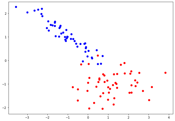
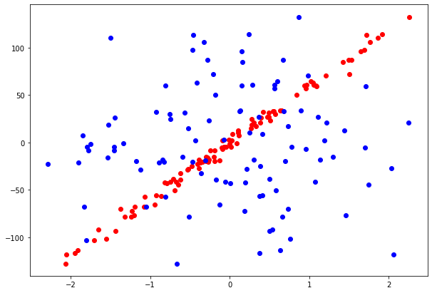
For each problem we generate datasets of 2 features and we visualize them. In the Classification problem both features are informative, while in Regression problem, only 1 of 2 features is an informative feature.
clf_data, clf_target = datasets.make_classification(n_features = 2, n_informative = 2, n_classes = 2,
                                                    n_redundant = 0, n_clusters_per_class = 1,
                                                    random_state = 7)
reg_data, reg_target = datasets.make_regression(n_features = 2, n_informative = 1, n_targets = 1,
                                                noise = 5., random_state = 7)
colors = ListedColormap(["red", "blue"])
pylab.scatter(clf_data[:,0], clf_data[:,1], c = clf_target, cmap = colors)
pylab.rcParams["figure.figsize"] = [10, 7]
pylab.scatter(reg_data[:,1], reg_target, color = "r")
pylab.scatter(reg_data[:,0], reg_target, color = "b")
pylab.rcParams["figure.figsize"] = [10, 7]
We split data into train and test sets.
clf_train_data, clf_test_data, clf_train_labels, clf_test_labels = model_selection.train_test_split(clf_data, clf_target,
                                                                                     test_size = 0.3, random_state = 1)
reg_train_data, reg_test_data, reg_train_labels, reg_test_labels = model_selection.train_test_split(reg_data, reg_target,
                                                                                     test_size = 0.3, random_state = 1)
Quality metrics in classification tasks
Classification model training
We’ll use SGDClassifier. It is a Linear classifier based on Stochastic gradient decent .
- Probabilistic classifier (Loss funciton: loss = ‘log’)
classifier = linear_model.SGDClassifier(loss = "log", random_state = 1, max_iter=1000)
classifier.fit(clf_train_data, clf_train_labels)
SGDClassifier(loss="log", random_state=1)
Generate classifier predicted labels:
predictions = classifier.predict(clf_test_data)
Generate a prediction in the form of the probability that the object belongs to the zero class or the first class.
probability_predictions = classifier.predict_proba(clf_test_data)
# original dataset labels
print(clf_test_labels)
[1 0 0 1 0 1 1 0 1 0 0 0 1 1 0 0 1 0 0 1 0 0 0 0 0 0 1 1 1 0]
# predicted labels
print(predictions)
[1 0 0 1 0 1 1 0 1 0 0 1 1 1 0 0 1 0 0 1 0 0 0 0 0 0 0 1 1 0]
Probabilities that the object belongs to the zero class or the first class.
The first probability is that object belongs to the the zero class and the second probability is that object belongs to the first class
print(probability_predictions[:10])
[[0.00000000e+00 1.00000000e+00]
 [9.99999997e-01 2.90779994e-09]
 [9.99990982e-01 9.01818055e-06]
 [0.00000000e+00 1.00000000e+00]
 [1.00000000e+00 7.01333183e-14]
 [5.16838702e-07 9.99999483e-01]
 [6.66133815e-16 1.00000000e+00]
 [1.00000000e+00 6.21822808e-13]
 [0.00000000e+00 1.00000000e+00]
 [9.99999998e-01 2.30155106e-09]]
We’ve done the preparational work. Now we come to the calculating metrics.
Accuracy
Accuracy is metric that shows closeness of the measurements to a specific value , designating a portion of correctly classified objects.
- pair[0] – correct label
- pair[1] – predicted label
- len(clf_test_labels) – data volume
# calculating thru Python means
acc1 = sum([1. if pair[0] == pair[1] else 0. for pair in zip(clf_test_labels, predictions)])/len(clf_test_labels)
# inbuilt accuracy score
acc2 = metrics.accuracy_score(clf_test_labels, predictions)
print (acc1, acc2)
0.9333333333333333 0.9333333333333333
Confusion matrix
Confusion matrix is the NxN matrix where N – number of classes (N=2 in our case). Confusion matrix provides to calculate many statistics metrics.
It shows the main characteristic of a built model:- True positive (TP) eqv. with hit
- True negative (TN) eqv. with correct rejection
- False positive (FP) eqv. with false alarm, type I error or underestimation
- False negative (FN) eqv. with miss, type II error or overestimation
matrix = metrics.confusion_matrix(clf_test_labels, predictions)
print("Confusion matrix\n",  matrix)
Confusion matrix
 [[17  1]
 [ 1 11]]
# manual calculations of True positives and True negatives
sum([1 if pair[0] == pair[1] else 0 for pair in zip(clf_test_labels, predictions)])
28
matrix.diagonal().sum()
28
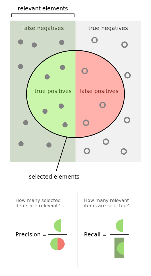
Precision
Precision describes the random errors, a measure of statistical variability.
First we estimate the accuracy of the classification to the zero class. We call the precision_score() function, pass it the correct class labels, the predicted class labels. And since by default our label is 1, we need to explicitly say that in this case we estimate the classification accuracy to the zero class. To do this, we use the pos_label argument and say that it is equal to 0 .
metrics.precision_score(clf_test_labels, predictions, pos_label = 0)
0.9444444444444444
We estimate the accuracy of the objects classification to the first class. Default pos_label = 1.
metrics.precision_score(clf_test_labels, predictions)
0.9230769230769231
Recall
See the Presision and Recall at a vivid picture:
metrics.recall_score(clf_test_labels, predictions, pos_label = 0)
0.9444444444444444
metrics.recall_score(clf_test_labels, predictions)
0.9166666666666666
metrics.f1_score(clf_test_labels, predictions, pos_label = 0)
0.9444444444444444
metrics.f1_score(clf_test_labels, predictions)
0.9166666666666666
Classification report
We use the classification_report function to get the summary table for each class.
print(metrics.classification_report(clf_test_labels, predictions))
              precision    recall  f1-score   support
           0       0.94      0.94      0.94        18
           1       0.92      0.92      0.92        12
    accuracy                           0.93        30
   macro avg       0.93      0.93      0.93        30
weighted avg       0.93      0.93      0.93        30
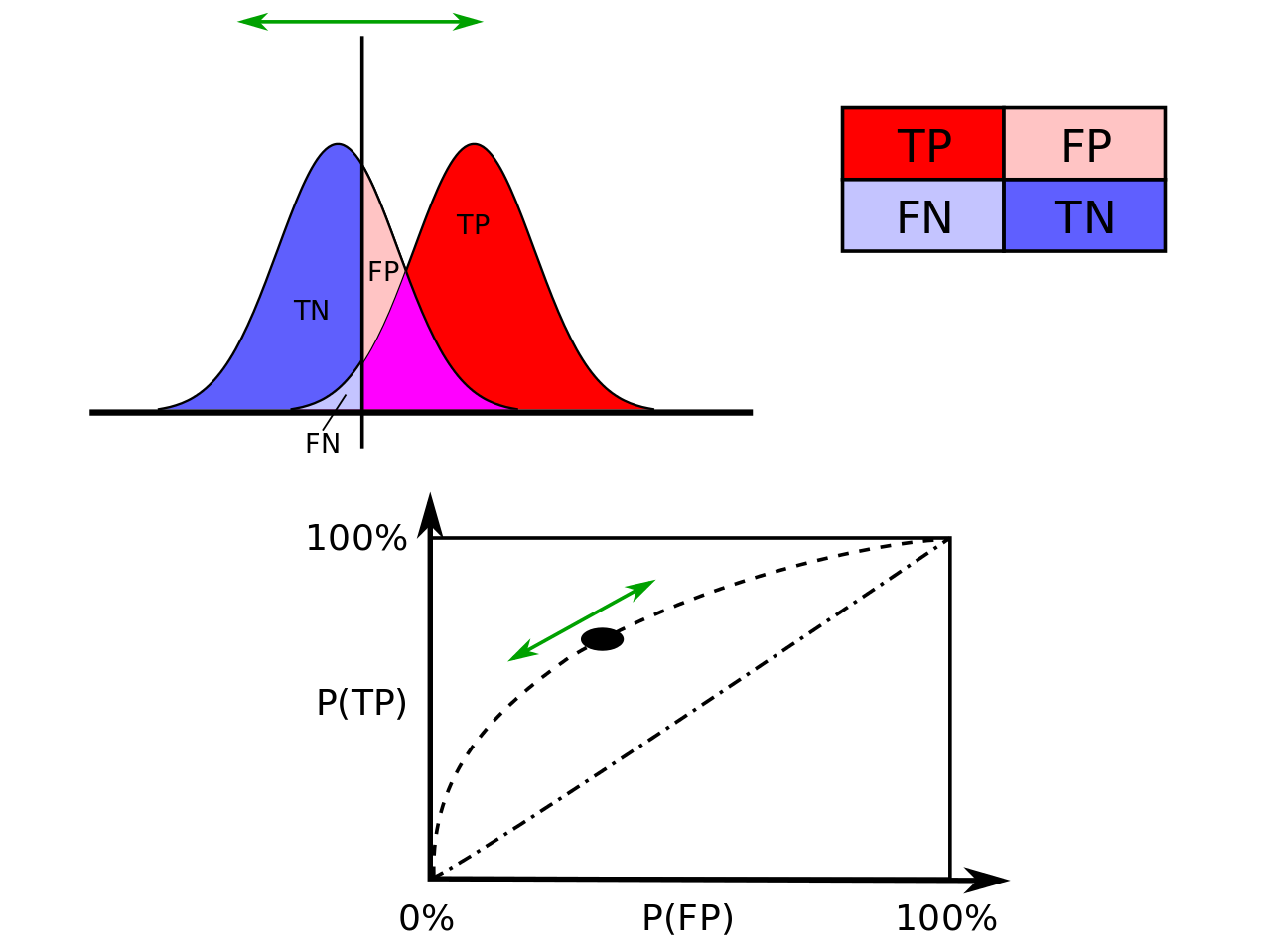
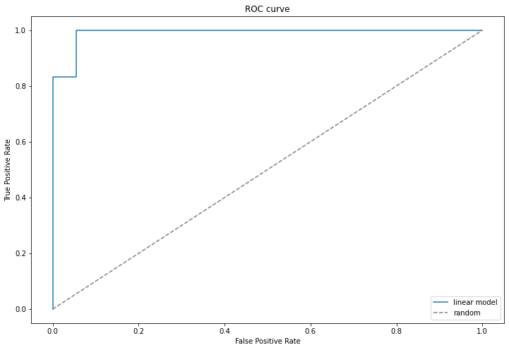
ROC curve – Receiver Operating Characteristic curve
An ROC curve plots TPR vs FPR at different classification thresholds. We use probability_predictions in our case.
- probability_predictions[:,1] is the probability that object is of the first class.
fpr, tpr, _ = metrics.roc_curve(clf_test_labels, probability_predictions[:,1])
# _ contains thresholds, we not using them
pylab.plot(fpr, tpr, label = "Linear model classifier")
pylab.plot([0, 1], [0, 1], "--", color = "grey", label = "Random classifier")
pylab.xlim([-0.05, 1.05])
pylab.ylim([-0.05, 1.05])
pylab.xlabel("False Positive Rate")
pylab.ylabel("True Positive Rate")
pylab.title("ROC curve")
pylab.legend(loc = "lower right")
pylab.rcParams["figure.figsize"] = [10, 7]
ROC AUC
ROC AUC shows a square area under the ROC function.
metrics.roc_auc_score(clf_test_labels, predictions)
0.9305555555555554
metrics.roc_auc_score(clf_test_labels, probability_predictions[:,1])
0.9907407407407407
PR AUC – Precision AUC
metrics.average_precision_score(clf_test_labels, predictions)
0.873611111111111
log_loss – logistical losses of Logistic regression
metrics.log_loss(clf_test_labels, probability_predictions[:,1])
0.21767621111290084
Metrics in the Regression problem
Training the regression model
regressor = linear_model.SGDRegressor(random_state = 1, max_iter = 20)
regressor.fit(reg_train_data, reg_train_labels)
SGDRegressor(max_iter=20, random_state=1)
reg_predictions = regressor.predict(reg_test_data)
print(reg_test_labels)
[   2.67799047    7.06525927  -56.43389936   10.08001896  -22.46817716
  -19.27471232   59.44372825  -21.60494574   32.54682713  -41.89798772
  -18.16390935   32.75688783   31.04095773    2.39589626   -5.04783924
  -70.20925097   86.69034305   18.50402992   32.31573461 -101.81138022
   15.14628858   29.49813932   97.282674     25.88034991  -41.63332253
  -92.11198201   86.7177122     2.13250832  -20.24967575  -27.32511755]
print(reg_predictions)
[ -1.46503565   5.75776789 -50.13234306   5.05646094 -24.09370893
  -8.34831546  61.77254998 -21.98350565  30.65112022 -39.25972497
 -17.19337022  30.94178225  26.98820076  -6.08321732  -3.46551
 -78.9843398   84.80190097  14.80638314  22.91302375 -89.63572717
  14.5954632   31.64431951  95.81031534  21.5037679  -43.1101736
 -95.06972123  86.70086546   0.47837761 -16.44594704 -22.72581879]
MAE – Mean Absolute Error
metrics.mean_absolute_error(reg_test_labels, reg_predictions)
3.748761311885298
MSE – Mean Squared Error
metrics.mean_squared_error(reg_test_labels, reg_predictions)
24.114925597460914
Mathematical Square Root of MSE
sqrt(metrics.mean_squared_error(reg_test_labels, reg_predictions))
4.91069502183356
Coefficient of determination – R2 score
The close R2 score to 1 the better/preciser model we have.
metrics.r2_score(reg_test_labels, reg_predictions)
0.989317615054695