The objective of the task is to build a model so that we can, as optimally as this data allows, relate molecular information, to an actual biological response.
We have shared the data in the comma separated values (CSV) format. Each row in this data set represents a molecule. The first column contains experimental data describing an actual biological response; the molecule was seen to elicit this response (1), or not (0). The remaining columns represent molecular descriptors (D1 through D1776), these are calculated properties that can capture some of the characteristics of the molecule – for example size, shape, or elemental constitution. The descriptor matrix has been normalized.
Data
Data description. We use the train.csv from the original task as bioresponse.csv file.
(1) sklearn.ensemble.RandomForestClassifier
and
(2) xgboost.XGBClassifier
from sklearn import ensemble, model_selection, metrics

import numpy as np
import pandas as pd
import xgboost as xgb
%pylab inline
Data
bioresponce = pd.read_csv("bioresponse.csv", header=0, sep=",")
bioresponce.head()
| Activity | D1 | D2 | D3 | D4 | D5 | D6 | D7 | D8 | D9 | … | D1767 | D1768 | D1769 | D1770 | D1771 | D1772 | D1773 | D1774 | D1775 | D1776 | |
|---|---|---|---|---|---|---|---|---|---|---|---|---|---|---|---|---|---|---|---|---|---|
| 0 | 1 | 0.000000 | 0.497009 | 0.10 | 0.0 | 0.132956 | 0.678031 | 0.273166 | 0.585445 | 0.743663 | … | 0 | 0 | 0 | 0 | 0 | 0 | 0 | 0 | 0 | 0 |
| 1 | 1 | 0.366667 | 0.606291 | 0.05 | 0.0 | 0.111209 | 0.803455 | 0.106105 | 0.411754 | 0.836582 | … | 1 | 1 | 1 | 1 | 0 | 1 | 0 | 0 | 1 | 0 |
| 2 | 1 | 0.033300 | 0.480124 | 0.00 | 0.0 | 0.209791 | 0.610350 | 0.356453 | 0.517720 | 0.679051 | … | 0 | 0 | 0 | 0 | 0 | 0 | 0 | 0 | 0 | 0 |
| 3 | 1 | 0.000000 | 0.538825 | 0.00 | 0.5 | 0.196344 | 0.724230 | 0.235606 | 0.288764 | 0.805110 | … | 0 | 0 | 0 | 0 | 0 | 0 | 0 | 0 | 0 | 0 |
| 4 | 0 | 0.100000 | 0.517794 | 0.00 | 0.0 | 0.494734 | 0.781422 | 0.154361 | 0.303809 | 0.812646 | … | 0 | 0 | 0 | 0 | 0 | 0 | 0 | 0 | 0 | 0 |
5 rows × 1777 columns
bioresponce_target = bioresponce.Activity.values
bioresponce_data = bioresponce.iloc[:, 1:]
Now we’ll run algorithms measuring their quality depending on the number of trees
Model RandomForestClassifier
We want to know how does the quality (accuracy) changes from the number of trees.
n_trees = [1] + list(range(10, 55, 5))
n_trees
[1, 10, 15, 20, 25, 30, 35, 40, 45, 50]%%time
scoring = []
for n_tree in n_trees:
estimator = ensemble.RandomForestClassifier(n_estimators = n_tree, min_samples_split=5, random_state=1)
score = model_selection.cross_val_score(estimator, bioresponce_data, bioresponce_target,
scoring = "accuracy", cv = 3)
scoring.append(score)
scoring = np.asmatrix(scoring)
Wall time: 20.6 s
The result is the matrix where each line corresponds to the number of trees from the n_trees array
scoring
matrix([[0.66906475, 0.668     , 0.6704    ],
        [0.75859313, 0.7592    , 0.7504    ],
        [0.78097522, 0.7616    , 0.7592    ],
        [0.78417266, 0.7736    , 0.7648    ],
        [0.78257394, 0.7736    , 0.7704    ],
        [0.78816946, 0.7752    , 0.7736    ],
        [0.78816946, 0.7856    , 0.7776    ],
        [0.78896882, 0.78      , 0.7832    ],
        [0.78976819, 0.7856    , 0.7896    ],
        [0.79536371, 0.7816    , 0.7928    ]])
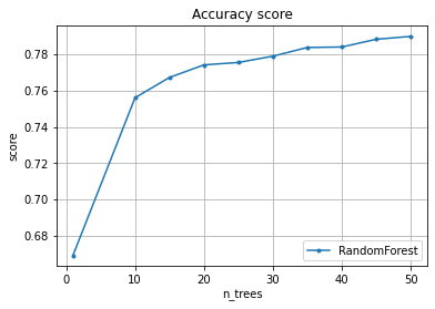
We draw a graph of scoring depending on the number of trees (n_trees).
pylab.plot(n_trees, scoring.mean(axis = 1), marker=".", label="RandomForest")
pylab.grid(True) # adding the grid to the graph
pylab.xlabel("n_trees")
pylab.ylabel("score")
pylab.title("Accuracy score")
pylab.legend(loc="lower right")
Model xgboost.XGBClassifier
Now we build the gradien boosting, xgb.XGBClassifier, and use the same set of max number of trees
Learning curves for trees of greater depth
- max_depth – max tree depth
- n_estimators – max number of trees
%%time
xgb_scoring = []
for n_tree in n_trees:
    estimator = xgb.XGBClassifier(learning_rate=0.1, max_depth=5, n_estimators=n_tree, min_child_weight=3)
    # the object xgb.XGBClassifier() is complient with cross_val_score() function
    score = model_selection.cross_val_score(estimator, bioresponce_data, bioresponce_target,
                                             scoring = "accuracy", cv = 3)
    xgb_scoring.append(score)
xgb_scoring = np.asmatrix(xgb_scoring)
Wall time: 1 min 48 s
matrix([[0.76498801, 0.756     , 0.756     ],
        [0.77617906, 0.7752    , 0.7688    ],
        [0.77857714, 0.7744    , 0.7768    ],
        [0.7873701 , 0.7784    , 0.7768    ],
        [0.79216627, 0.7736    , 0.7832    ],
        [0.79776179, 0.7776    , 0.7824    ],
        [0.79616307, 0.7816    , 0.78      ],
        [0.79296563, 0.7848    , 0.7792    ],
        [0.79856115, 0.7832    , 0.7808    ],
        [0.79936051, 0.7832    , 0.7832    ]])
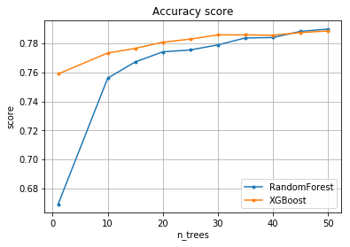
We draw a grath with both RF and the Gradient boosting for comparison.
pylab.plot(n_trees, scoring.mean(axis = 1), marker=".", label="RandomForest")
pylab.plot(n_trees, xgb_scoring.mean(axis = 1), marker=".", label="XGBoost")
pylab.grid(True)
pylab.xlabel("n_trees")
pylab.ylabel("score")
pylab.title("Accuracy score")
pylab.legend(loc="lower right")
Results comparison
| Classifier algorithm | Timing | Best accuracy |
|---|---|---|
| Random Forest | 20 sec. | 0.8 |
| Gradient boosting | 108 sec. | 0.8 |
Consclusion
- Both algorithms are of high quality/accuracy, 0.8.
- Gradient boosting yields relatively high classification results with a low number of max trees compare to RF.
- Random Forest algorithm is much faster than that of Gradient boosting, XGBoost. See the results comparison table above.