We show how to work with Decision trees at the Sklearn library.
Sklearn.tree; Sklearn tree examples
from matplotlib.colors import ListedColormap
from sklearn import model_selection, datasets, metrics, tree

import numpy as np
%pylab inline
Data generation
We will solve the problem of multi-class classification. For that we generate data from sklearn datasets: 3 classes with 2 features each. These features will be shown as x and y coordinates.
classification_problem = datasets.make_classification(
    n_features = 2, n_informative = 2,
    n_classes = 3, n_redundant=0,
    n_clusters_per_class=1, random_state=3)
# features
print(classification_problem[0].shape)
classification_problem[0][:3]
(100, 2)
array([[ 2.21886651,  1.38263506],
       [ 2.07169996, -1.07356824],
       [-1.93977262, -0.85055602]])
# let"s output labels (targets)
classification_problem[1]
array([0, 1, 2, 0, 0, 2, 0, 1, 0, 1, 0, 0, 1, 1, 2, 1, 1, 1, 1, 0, 1, 2,
       2, 1, 1, 0, 2, 1, 2, 2, 1, 1, 1, 0, 0, 0, 1, 1, 0, 2, 2, 0, 0, 2,
       0, 1, 2, 2, 0, 0, 2, 2, 2, 0, 2, 2, 2, 1, 1, 2, 0, 1, 0, 1, 2, 0,
       0, 2, 2, 0, 0, 2, 0, 0, 0, 2, 1, 0, 1, 2, 0, 1, 0, 0, 0, 2, 0, 2,
       1, 2, 0, 1, 2, 1, 1, 1, 1, 2, 0, 2])
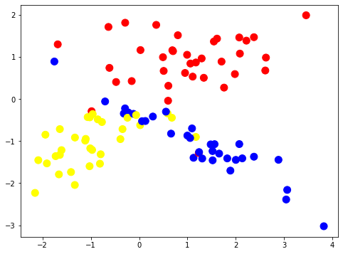
We plot out the colored dataset labels on the 2 features surface, x, y.
# colormap list for the classes dataset (as marks/dots)
colors = ListedColormap(["red", "blue", "yellow"])
# colormaps for the building of dividing surfaces
light_colors = ListedColormap(["lightcoral", "lightblue", "lightyellow"])
pylab.figure(figsize=(8,6))
pylab.scatter(list(map(lambda x: x[0], classification_problem[0])), list(map(lambda x: x[1], classification_problem[0])),
              c=classification_problem[1], cmap=colors, s=100)
Split dataset for train and test subsets.
train_data, test_data, train_labels, test_labels = model_selection.train_test_split(
 classification_problem[0],
 classification_problem[1],
 test_size = 0.3,
 random_state = 1)
clf = tree.DecisionTreeClassifier(random_state=1)
clf.fit(train_data, train_labels)
DecisionTreeClassifier(random_state=1)
predictions = clf.predict(test_data)
metrics.accuracy_score(test_labels, predictions)
0.7666666666666667
predictions
array([0, 0, 0, 0, 0, 1, 1, 0, 0, 0, 2, 2, 2, 2, 2, 1, 0, 1, 0, 2, 2, 0,
       2, 0, 0, 0, 2, 1, 2, 0])
def get_meshgrid(data, step=.05, border=.5,):
    x_min, x_max = data[:, 0].min() - border, data[:, 0].max() + border
    y_min, y_max = data[:, 1].min() - border, data[:, 1].max() + border
    return np.meshgrid(np.arange(x_min, x_max, step), np.arange(y_min, y_max, step))
def plot_decision_surface(estimator, train_data, train_labels, test_data, test_labels,
                          colors = colors, light_colors = light_colors):
    #fit model
    estimator.fit(train_data, train_labels)

    #set figure size
    pyplot.figure(figsize = (16, 6))

    # plot decision surface on the train data
    pyplot.subplot(1,2,1)
    xx, yy = get_meshgrid(train_data)
    mesh_predictions = np.array(estimator.predict(np.c_[xx.ravel(), yy.ravel()])).reshape(xx.shape)
    # draw the dividing surface
    pyplot.pcolormesh(xx, yy, mesh_predictions, cmap = light_colors)
    # above the surfaces we put the class labels (train data)
    pyplot.scatter(train_data[:, 0], train_data[:, 1], c = train_labels, s = 100, cmap = colors)
    pyplot.title("Train data, accuracy={:.2f}".format(metrics.accuracy_score(train_labels, estimator.predict(train_data))))

    # plot decision surface on the test data
    pyplot.subplot(1,2,2)
    pyplot.pcolormesh(xx, yy, mesh_predictions, cmap = light_colors)
    pyplot.scatter(test_data[:, 0], test_data[:, 1], c = test_labels, s = 100, cmap = colors)
    pyplot.title("Test data, accuracy={:.2f}".format(metrics.accuracy_score(test_labels, estimator.predict(test_data))))
Decision trees
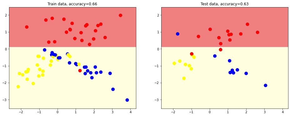
We generate simple decision tree with max depth = 1
# simple decision tree with max depth = 1
estimator = tree.DecisionTreeClassifier(random_state = 1, max_depth = 1)

plot_decision_surface(estimator, train_data, train_labels, test_data, test_labels)
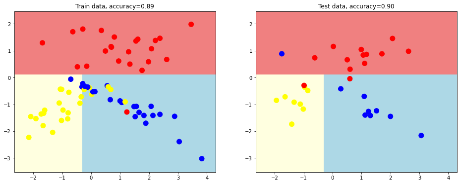
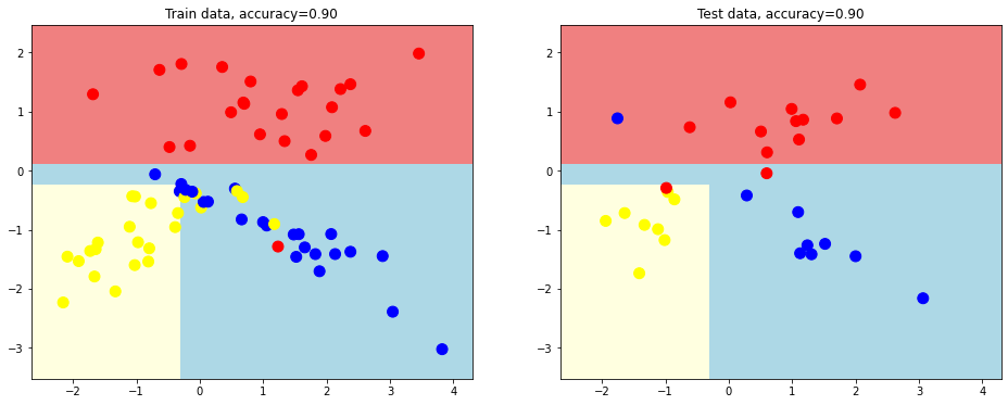
We now creare a better desition tree with depth 2.
# we build decision tree of depth=2 and plot out the dividing surfaces
plot_decision_surface(tree.DecisionTreeClassifier(random_state = 1, max_depth = 2),
                      train_data, train_labels, test_data, test_labels)
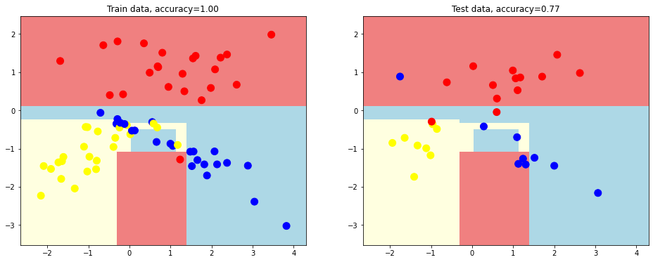
We creare another desition tree with depth equal 3.
# tree depth = 3
plot_decision_surface(tree.DecisionTreeClassifier(random_state = 1, max_depth = 3),
                      train_data, train_labels, test_data, test_labels)
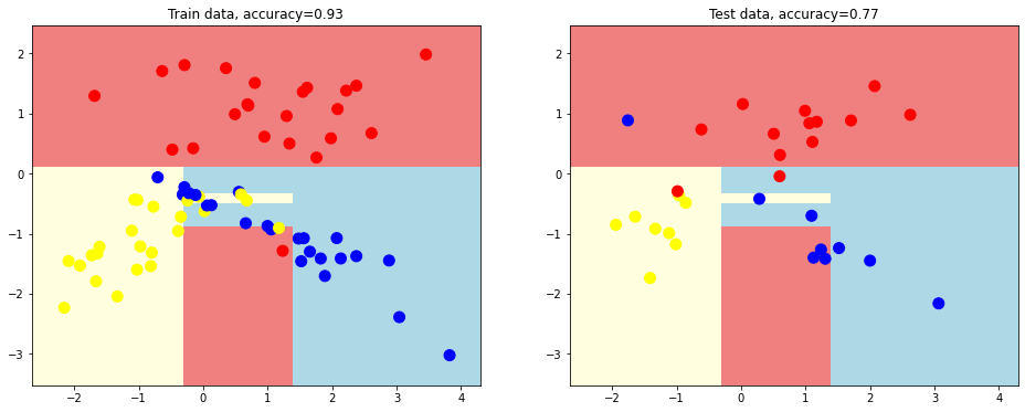
# dividing surfaces without decision tree depth limit
plot_decision_surface(tree.DecisionTreeClassifier(random_state = 1),
                      train_data, train_labels, test_data, test_labels)
This kind of decision tree looks overfitting.
Solve overfitting
Let’s try to solve overfitting. We define the minimum objects (samples) at the leaf node: min_samples_leaf = 3
plot_decision_surface(tree.DecisionTreeClassifier(random_state = 1, min_samples_leaf = 3),
                      train_data, train_labels, test_data, test_labels)