The objective of the task is to build a model so that we can, as optimally as this data allows, relate molecular information, to an actual biological response.
We have shared the data in the comma separated values (CSV) format. Each row in this data set represents a molecule. The first column contains experimental data describing an actual biological response; the molecule was seen to elicit this response (1), or not (0). The remaining columns represent molecular descriptors (D1 through D1776), these are calculated properties that can capture some of the characteristics of the molecule – for example size, shape, or elemental constitution. The descriptor matrix has been normalized.
Data
Data description. We use the train.csv from the original task as bioresponse.csv file.
%pylab inline
from sklearn import ensemble, model_selection, metrics
import numpy as np
import pandas as pd
bioresponce = pd.read_csv("bioresponse.csv", header=0, sep=",")
bioresponce.head()
| Activity | D1 | D2 | D3 | D4 | D5 | D6 | D7 | D8 | D9 | … | D1767 | D1768 | D1769 | D1770 | D1771 | D1772 | D1773 | D1774 | D1775 | D1776 | |
|---|---|---|---|---|---|---|---|---|---|---|---|---|---|---|---|---|---|---|---|---|---|
| 0 | 1 | 0.000000 | 0.497009 | 0.10 | 0.0 | 0.132956 | 0.678031 | 0.273166 | 0.585445 | 0.743663 | … | 0 | 0 | 0 | 0 | 0 | 0 | 0 | 0 | 0 | 0 |
| 1 | 1 | 0.366667 | 0.606291 | 0.05 | 0.0 | 0.111209 | 0.803455 | 0.106105 | 0.411754 | 0.836582 | … | 1 | 1 | 1 | 1 | 0 | 1 | 0 | 0 | 1 | 0 |
| 2 | 1 | 0.033300 | 0.480124 | 0.00 | 0.0 | 0.209791 | 0.610350 | 0.356453 | 0.517720 | 0.679051 | … | 0 | 0 | 0 | 0 | 0 | 0 | 0 | 0 | 0 | 0 |
| 3 | 1 | 0.000000 | 0.538825 | 0.00 | 0.5 | 0.196344 | 0.724230 | 0.235606 | 0.288764 | 0.805110 | … | 0 | 0 | 0 | 0 | 0 | 0 | 0 | 0 | 0 | 0 |
| 4 | 0 | 0.100000 | 0.517794 | 0.00 | 0.0 | 0.494734 | 0.781422 | 0.154361 | 0.303809 | 0.812646 | … | 0 | 0 | 0 | 0 | 0 | 0 | 0 | 0 | 0 | 0 |
5 rows × 1777 columns
bioresponce.shape
(3751, 1777)
bioresponce.columns
Index(["Activity", "D1", "D2", "D3", "D4", "D5", "D6", "D7", "D8", "D9",
       ...
       "D1767", "D1768", "D1769", "D1770", "D1771", "D1772", "D1773", "D1774",
       "D1775", "D1776"],
      dtype="object", length=1777)
bioresponce_target = bioresponce.Activity.values
print("bioresponse = 1: {:.2f}\nbioresponse = 0: {:.2f}".format(sum(bioresponce_target)/float(len(bioresponce_target)),
                1.0 - sum(bioresponce_target)/float(len(bioresponce_target))))
bioresponse = 1: 0.54
bioresponse = 0: 0.46
From the classes amount we see that the classification task is almost balanced.
Now we cut data off the targets:
bioresponce_data = bioresponce.iloc[:, 1:]
We use RandomForestClassifier with needed parameters. We may train and apply the model using fit() and predict() methods. The model estimation we may do with Exhaustive Grid Search or Randomized Grid Search. We do not do it here. You might see its implementation in here.
Here we analyse the model quality/presision dependence on the train objects amount.
Learning curves for small depth trees
We build the Random Forest model for 50 trees each having max depth = 2.
rf_classifier_low_depth = ensemble.RandomForestClassifier(
n_estimators = 50, max_depth = 2, random_state = 1)
The function learning_curve() allows to show the presision dependence on the training objects amount. It takes algorithm, targets, data and the proportion with witch we want to be trained.
Wit the learning_curve() method several models will be built, we get quality metric (scoring) for each one. And the method will return us the size of train set, quality scoring on train and on test.
Having those data we may ananlyse how the model quality changes/depends on the train set size.
train_sizes, train_scores, test_scores = model_selection.learning_curve(
rf_classifier_low_depth, bioresponce_data, bioresponce_target,                                                                        train_sizes=np.arange(0.1,1., 0.2),
cv=3, scoring="accuracy")
np.arange(0.1, 1., 0.2) # [0.1, 0.3, 0.5, 0.7, 0.9]
print(train_sizes)
# we take mean for all CV folds.
print(train_scores.mean(axis = 1))
print(test_scores.mean(axis = 1))
[ 250 750 1250 1750 2250 ]
[0.74933333 0.71333333 0.68453333 0.69104762 0.69022222]
[0.62356685 0.64195598 0.65369955 0.66248974 0.66728527]
pylab.grid(True)
pylab.plot(train_sizes, train_scores.mean(axis = 1), "g-", marker="o", label="train")
pylab.plot(train_sizes, test_scores.mean(axis = 1), "r-", marker="o", label="test")
pylab.ylim((0.0, 1.05))
pylab.legend(loc="lower right")
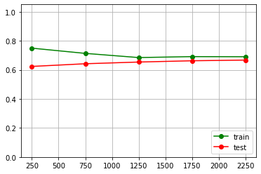
The conclusion of those data
The further growth of train set size (over 2250 items) will not influence the model quality.
Learning curves for trees of greater depth
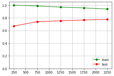
We’ll try to increase the model difficulty, this might increase its quality metrics. Let’s set max_depth = 10.
rf_classifier = ensemble.RandomForestClassifier(
n_estimators = 50, max_depth = 10, random_state = 1)
train_sizes, train_scores, test_scores =
model_selection.learning_curve(rf_classifier,
 bioresponce_data, bioresponce_target,
 train_sizes=np.arange(0.1,1, 0.2),
cv=3, scoring="accuracy")
pylab.grid(True)
pylab.plot(train_sizes, train_scores.mean(axis = 1), "g-", marker="o", label="train")
pylab.plot(train_sizes, test_scores.mean(axis = 1), "r-", marker="o", label="test")
pylab.ylim((0.0, 1.05))
pylab.legend(loc="lower right")