Design patterns for hierarchical data storage and effective processing

The hierarchical data storage problem is a non-trivial task in relational database context. For example, your online shop has goods of different categories and subcategories creating tree spans for 5 levels. How should they be stored in a database?

Luckily, there are several approaches (design patterns) that will help the developer to design database structure without both odd tables and code. As a result, the site will work faster and any changes, even on database layer, won’t cause troubles. We will study these approaches below.

Adjacency List

This design pattern is the simplest solution to store and work with hierarchical data structures. Below you can see what it looks like:

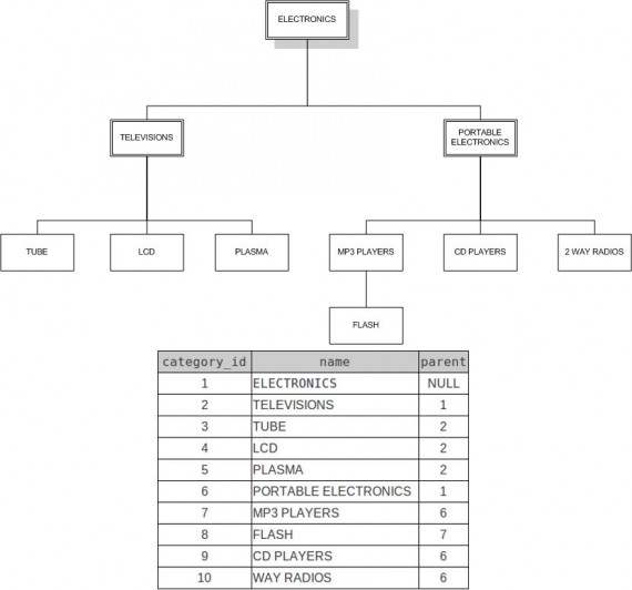
Quite simple, isn’t it? The only thing needed is to add some explanatory statements to furnish a thorough understanding of the adjacency list:

• Parent_id is a foreign key which is connected to category_id.
• The no-children nodes are called leaf nodes. The children and grandchildren are called descendants, and parents with grandparents are ancestors. Root node is an element that has no parents. In our case, it is an Electronics element.

 The last comment is valid for every design pattern which will be mentioned in this article. Now, let’s create a table to see how an adjacency list works in practice.

CREATE TABLE category_adj ( 
    id int unsigned NOT NULL AUTO_INCREMENT, 
    name varchar(25) NOT NULL, 
    parent_id int unsigned DEFAULT NULL,
    PRIMARY KEY (id), 
    FOREIGN KEY (parent_id) REFERENCES category_adj (id) ON DELETE CASCADE ON UPDATE CASCADE 
)

Note, we use the foreign key with ON DELETE CASCADE ON UPDATE CASCADE – it allows deleting and updating foreign key values.

Firstly, we add a root node element:

INSERT INTO category_adj(name,parent_id) VALUES ('Electronics',NULL)

After that, we can add the root node’s descendants

INSERT INTO category_adj(name,parent_id) VALUES('Televisions',1)
INSERT INTO category_adj(name,parent_id) VALUES('Portable electronics',1)

And the next levels:

INSERT INTO category_adj(name,parent_id) VALUES('Tube',2)
INSERT INTO category_adj(name,parent_id) VALUES('LCD',2)
INSERT INTO category_adj(name,parent_id) VALUES('Plasma',2)
INSERT INTO category_adj(name,parent_id) VALUES('MP3 Players',3)
INSERT INTO category_adj(name,parent_id) VALUES('CD Palyers',3)
INSERT INTO category_adj(name,parent_id) VALUES('2 Way radios',3)
INSERT INTO category_adj(name,parent_id) VALUES('FLASH',7)

The listing shows how we realize the structure on picture 1. As you can see, there is nothing hard at all. All we need is to insert values with the right parent_id.

Now let’s consider approaches for how to use some specific operations in a context of an adjacency list.

To get the root element:

SELECT id, name FROM category_adj WHERE parent_id IS NULL

The result is:

Finding Television’s children:

SELECT id, name FROM category_adj WHERE parent_id = 2

Here they are:

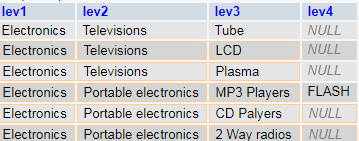
Let’s go to more engaging operations. To unfold the full tree we need:

SELECT c1.name AS level1, c2.name as level2, c3.name as level3, c4.name as level4
FROM category_adj AS c1
LEFT JOIN category_adj AS c2 ON c2.parent_id = c1.id
LEFT JOIN category_adj AS c3 ON c3.parent_id = c2.id
LEFT JOIN category_adj AS c4 ON c4.parent_id = c3.id WHERE c1.name ='Electronics'

Self-join unfolds the full tree. As a result we have:

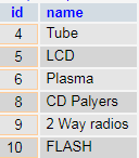
And the last example – getting all leaf nodes. The leaf nodes are elements which have no children.

SELECT c1.id, c1.name FROM category_adj c1 
LEFT JOIN category_adj c2 ON c2.parent_id = c1.id
WHERE c2.id IS NULL

And here are all our no-children elements:

So, if you are creating tree-structured data, an adjacency list is a convenient pattern to ease your DB design process.

Materialized Path

This design pattern is usually used for the realization of a comment system on a website. Why is it convenient to use a materialized path? Let’s create a comment table and look into the matter:

CREATE TABLE comment (
   id int NOT NULL AUTO_INCREMENT,
   comment varchar(30) NOT NULL,
   path varchar(30) NOT NULL,
   PRIMARY KEY (`id`)
);

INSERT INTO comment (id, comment, path) VALUES (NULL, 'Nice article', '/1/');
SET @COMMENT_ID = LAST_INSERT_ID();
UPDATE comment SET path = CONCAT('/', @COMMENT_ID, '/') WHERE id = @COMMENT_ID;
INSERT INTO comment (id, comment, path) VALUES (NULL, 'wow!', '');
SET @COMMENT1_ID = LAST_INSERT_ID();
UPDATE comment SET path = CONCAT('/', @COMMENT_ID, '/', @COMMENT1_ID, '/') WHERE id = @COMMENT1_ID;
INSERT INTO comment (id, comment, path) VALUES (NULL, 'really nice', '');
SET @COMMENT2_ID = LAST_INSERT_ID();
UPDATE comment SET path = CONCAT('/', @COMMENT_ID, '/', @COMMENT2_ID, '/') WHERE id = @COMMENT2_ID;
INSERT INTO comment (id, comment, path) VALUES (NULL, 'super', '');
SET @COMMENT1_1_ID = LAST_INSERT_ID();
UPDATE comment SET path = CONCAT('/', @COMMENT_ID, '/', @COMMENT1_ID, '/', @COMMENT1_1_ID, '/') WHERE id = @COMMENT1_1_ID;
INSERT INTO comment (id, comment, path) VALUES (NULL, 'good', '');
SET @COMMENT2_1_ID = LAST_INSERT_ID();
UPDATE comment SET path = CONCAT('/', @COMMENT_ID, '/', @COMMENT2_ID, '/', @COMMENT2_1_ID, '/') WHERE id = @COMMENT2_1_ID;

In the insertions listed above, we add new comments and paths that show the hierarchy of comments.

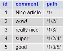
For example, path 1/3/5 equals Nice article->really nice->good

To get all comments that are related to 1/3/[value] hierarchy:

SELECT * FROM comment WHERE path LIKE '/1/3/%' ORDER BY path ASC

To delete the hierarchy which starts with “wow” comment

DELETE FROM comment WHERE path LIKE '/1/2/%'

Result:

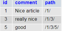
Materialized Path, or path enumeration, isn’t the best choice to use with relational databases. In the MongoDB database it works more easily and doesn’t look as frightful as in the examples above.

Nested sets

Another approach in building hierarchical structures is Nested sets. The main pattern attribute is the presence of left key and right key. The main advantage of nested sets is data selection speed. Main disadvantage – changes in the DB are time-consuming, because it’s necessary to change left and right keys.

To demonstrate the basic capabilities of nested sets, we will create a tree table and fill it with data:

CREATE TABLE `tree` (
 `id` int NOT NULL AUTO_INCREMENT,
 `branch` varchar(30) NOT NULL,
 `lft` int NOT NULL,
 `rgt` int NOT NULL,
 PRIMARY KEY (`id`)
);

INSERT INTO tree (id, branch, lft, rgt) VALUES (NULL, 'main_branch1', 1, 28);
INSERT INTO tree (id, branch, lft, rgt) VALUES (NULL, 'sub_bracnh2_1', 2, 15);
INSERT INTO tree (id, branch, lft, rgt) VALUES (NULL, 'sub_bracnh2_2', 16, 27);
INSERT INTO tree (id, branch, lft, rgt) VALUES (NULL, 'sub_bracnh3_1', 3, 8);
INSERT INTO tree (id, branch, lft, rgt) VALUES (NULL, 'sub_bracnh3_2', 9, 14);
INSERT INTO tree (id, branch, lft, rgt) VALUES (NULL, 'sub_bracnh3_3', 17, 18);
INSERT INTO tree (id, branch, lft, rgt) VALUES (NULL, 'sub_bracnh3_4', 19, 26);
INSERT INTO tree (id, branch, lft, rgt) VALUES (NULL, 'sub_bracnh4_1', 4, 5);
INSERT INTO tree (id, branch, lft, rgt) VALUES (NULL, 'sub_bracnh4_2', 6, 7);
INSERT INTO tree (id, branch, lft, rgt) VALUES (NULL, 'sub_bracnh4_3', 10, 11);
INSERT INTO tree (id, branch, lft, rgt) VALUES (NULL, 'sub_bracnh4_4', 12, 13);
INSERT INTO tree (id, branch, lft, rgt) VALUES (NULL, 'sub_branch_4_5', 20, 21);
INSERT INTO tree (id, branch, lft, rgt) VALUES (NULL, 'sub_branch_4_6', 22, 23);
INSERT INTO tree (id, branch, lft, rgt) VALUES (NULL, 'sub_branch_4_7', 24, 25);

At first glance, it can be hard to understand what the values of keys rgt and lft mean. Suppose the root elements are lft = 1 and rgt = 28. It means that number of elements equals 28/2 = 14 (the golden rule is that the root’s rgt value is always a double of the total number of nodes in DB).

The root elements lft = 1 and rgt = 28, and all child elements in the range lft >1 and rgt < 28 belong to the main_branch1 element. This works for other elements (in an example below you will see what it looks like).

SELECT * FROM tree WHERE lft BETWEEN 2 AND 15

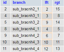
Retrieving data from our tree by nested sets is much easier than in the Adjacency list. We avoid lots of JOINs when using Nested sets. The SQL request below is more expanded compared to the SQL query above, but it’s easier in use to select the needed values:

SELECT children.* FROM tree parent JOIN tree children ON children.lft BETWEEN parent.lft AND parent.rgt WHERE parent.id = 3

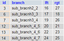
See, how easy the selection of data in hierarchic structures can be. Now we are going to the last design pattern – Closure Table.

Closure table

One of the most popular and cross functional ways to store hierarchic structures in a relational database is the Closure table. A simple and elegant solution that allows you to work with tables without extra harassment and to enjoy the process.

Instead of the concepts listed above, the Closure table works by using two tables. The first table will store basic information, while the second stores the connections between entities (ancestor-descendant relations).

Basic table:

CREATE TABLE family (
   id INT NOT NULL AUTO_INCREMENT,
   role VARCHAR(250) NOT NULL,
   PRIMARY KEY(id)
)

Relations table:

CREATE TABLE relation (
  ancestor_id INT NOT NULL,
  descendant_id INT NOT NULL,
  depth INT NOT NULL,
  PRIMARY KEY (ancestor_id, descendant_id)
)

Adding needed data:

INSERT INTO family VALUES (NULL, 'parents');
SET @PARENTS = LAST_INSERT_ID();
INSERT INTO family VALUES (NULL, 'daughter');
SET @DAUGHTER = LAST_INSERT_ID();
INSERT INTO family VALUES (NULL, 'son');
SET @SON = LAST_INSERT_ID();
INSERT INTO family VALUES (NULL, 'grandchild (daughter\'s side)');
SET @DAU_GRAND2 = LAST_INSERT_ID();
INSERT INTO family VALUES (NULL, 'grandchild (son\'s side)');
SET @SON_GRAND1 = LAST_INSERT_ID();
INSERT INTO family VALUES (NULL, 'grandchild (son\'s side)');
SET @SON_GRAND2 = LAST_INSERT_ID();
INSERT INTO family VALUES (NULL, 'great grandchildren (son\'s side) ');
SET @SON_GRAND1_GREAT1 = LAST_INSERT_ID();
INSERT INTO family VALUES (NULL, 'great grandchildren (son\'s side) ');
SET @SON_GRAND1_GREAT2 = LAST_INSERT_ID();
INSERT INTO relation VALUES (@PARENTS, @PARENTS, 0);
INSERT INTO relation VALUES (@PARENTS, @DAUGHTER, 1);
INSERT INTO relation VALUES (@PARENTS, @SON, 1);
INSERT INTO relation VALUES (@PARENTS, @DAU_GRAND1, 2);
INSERT INTO relation VALUES (@PARENTS, @DAU_GRAND2, 2);
INSERT INTO relation VALUES (@PARENTS, @SON_GRAND1, 2);
INSERT INTO relation VALUES (@PARENTS, @SON_GRAND2, 2);
INSERT INTO relation VALUES (@PARENTS, @SON_GRAND1_GREAT1, 3);
INSERT INTO relation VALUES (@PARENTS, @SON_GRAND1_GREAT2, 3);
INSERT INTO relation VALUES (@DAUGHTER, @DAUGHTER, 0);
INSERT INTO relation VALUES (@DAUGHTER, @DAU_GRAND1, 1);
INSERT INTO relation VALUES (@DAUGHTER, @DAU_GRAND2, 1);
INSERT INTO relation VALUES (@SON, @SON, 0);
INSERT INTO relation VALUES (@SON, @SON_GRAND1, 1);
INSERT INTO relation VALUES (@SON, @SON_GRAND2, 1);
INSERT INTO relation VALUES (@SON, @SON_GRAND1_GREAT1, 2);
INSERT INTO relation VALUES (@SON, @SON_GRAND1_GREAT2, 2);
INSERT INTO relation VALUES (@DAU_GRAND1, @DAU_GRAND1, 0);
INSERT INTO relation VALUES (@DAU_GRAND2, @DAU_GRAND2, 0);
INSERT INTO relation VALUES (@SON_GRAND1, @SON_GRAND1, 0);
INSERT INTO relation VALUES (@SON_GRAND1, @SON_GRAND1_GREAT1, 1);
INSERT INTO relation VALUES (@SON_GRAND1, @SON_GRAND1_GREAT2, 1);
INSERT INTO relation VALUES (@SON_GRAND2, @SON_GRAND2, 0);
INSERT INTO relation VALUES (@SON_GRAND1_GREAT1, @SON_GRAND1_GREAT1, 0);
INSERT INTO relation VALUES (@SON_GRAND1_GREAT2, @SON_GRAND1_GREAT2, 0);

To read data, we join the family and relation tables. Thanks to the relation @SON-@SON we are able to get all the son’s side members including their ancestor:

SELECT f.* FROM family f JOIN relation r ON f.id = r.descendant_id WHERE r.ancestor_id = 3

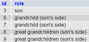
If we don’t want to get ancestor, we can simply add r.depth > 0

SELECT f.* FROM family f JOIN relation r ON f.id = r.descendant_id WHERE r.ancestor_id = 3 AND r.depth > 0

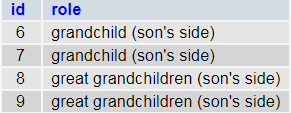
Developers all over the world strongly recommend using a Closure table, because it’s easy both in understanding and use. Now we will compare all approaches to find the best solution.

Making the best decision

After considering each concept, we are able to compare and find the best design pattern. As the first step, let’s highlight the main demands for each design pattern for hierarchical data:

• Minimal number of requests (for example, we want to use only one query to get branch)
• High-performance and low request runtime
• Data validity
• Convenient working with MySQL. It is the most popular DBMS which, unfortunately, doesn’t support recursion, and it would be good if the purchased concept furnishes us with reliable service.

The table below shows which hierarchical data storage concept is most convenient and reliable:

So, Closure table is the best option. Of course, it has its own disadvantages, but in fact, considering a developer’s basic needs, Closure table would be a right variant for everyone who wants to implement the hierarchical structure in his project. More about considered concepts you can read in the book SQL Antipatterns: Avoiding the Pitfalls of Database Programming (pdf).