from matplotlib.colors import ListedColormap
from sklearn import model_selection, datasets, linear_model, metrics
import numpy as np

%pylab inline
  

Linear regression models

Data generation

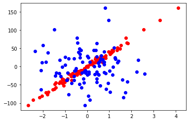
We build a dataset with 2 features: one is informative and the other is redundant. Besides, when adding coef=True we ask to return us also the approximation function coefficients into the coef array.

data, target, coef = datasets.make_regression\
	(n_features = 2, n_informative = 1, n_targets = 1, 
         noise = 5., coef = True, random_state = 2)
  

print("Coefficients:" , coef, "intercept:" , linear_regressor.intercept_)
  

Coefficients: [38.07925 0.000] intercept: -0.130524679653

We plot the target, y, dependence of features: x₁, x₂.

pylab.scatter(data[:,0], target, color = r)
pylab.scatter(data[:,1], target, color = b)
  

Based on the above plot one can find out which of 2 features is informative (red one).

Let’s build a model and view its coefficients.

We split data for train and test sets.

train_data, test_data, train_labels, test_labels = \
 model_selection.train_test_split(data, target, test_size = 0.3)
  

LinearRegression over the train data

We build a linear regressor model (L2 regularization) based on the given dataset. Later we’ll evaluate the model using cross-validation.

  # build a model
linear_regressor = linear_model.LinearRegression() 
  # train the model
linear_regressor.fit(train_data, train_labels)  
  # get the model predictions 
predictions = linear_regressor.predict(test_data)  
  

# original labels
print(test_labels)
  

[ -76.75213382   34.35183007  -11.18242389  -61.47026695   44.66274342
  -13.26392817   18.17188553   25.7124082   -19.16792315  101.14760598
 -105.77758163   23.87701013   12.42286854  -18.57607726   21.20540389
   38.36241814  -45.38589148   29.8208999   -84.32102748    0.34799656
   11.96165156   39.70663436   41.95683853  -10.06708677  -63.4056294
  -16.30914909  -45.27502383  -57.46293828   28.15553021  -17.27897399]
  

# predicted labels on the test objects
print(predictions)
  

[ -68.31690488   38.87063362  -12.62644748  -55.97354269   50.53828408
  -15.92863777   18.48923956   28.00480498  -10.77148765   95.936183
 -100.85245811   31.5152017     6.88671402  -24.57940803   16.71365889
   41.26798296  -43.31634025   31.48688292  -80.45697523   -1.51872908
   13.95215963   37.61637807   43.5105848    -9.47060759  -59.39279793
  -11.74032551  -47.34651564  -53.9339432    22.64507627  -13.03856029]
  

Let’s count MAE of those original dataset labels to the predicted labels.

metrics.mean_absolute_error(test_labels, predictions)
  

3.859435388011848

We use cross_val_score() to evaluate our linear regressor, the regressor evaluation will be more precise.

·Scoring is MAE (scoring = neg_mean_absolute_error).

·We cross-validate the data using 10 folds (cv = 10).

linear_scoring = model_selection.cross_val_score\
	(linear_regressor, data, target, scoring = neg_mean_absolute_error,  cv = 10)
print(mean: {}, std: {}.format(linear_scoring.mean(), linear_scoring.std()))
  

mean: -4.070071498779695, std: 1.0737104492890204

We create now our own scorer with parameter greater_is_better.

scorer = metrics.make_scorer(metrics.mean_absolute_error, greater_is_better = True)
  

And now we evaluate the model, linear_regressor.

linear_scoring = model_selection.cross_val_score\
	(linear_regressor, data, target, scoring=scorer,  cv = 10)
print(mean: {}, std: {}.format(linear_scoring.mean(), linear_scoring.std()))
  

mean: 4.070071498779695, std: 1.0737104492890204

Let’s take a look at the coefficients of the inbuilt dataset. We’ve got them from the make_regression() function.

coef
  

array([38.07925837, 0.0])

The coefficients of the model built with LinearRegression():

linear_regressor.coef_ 
  

array([37.86162519, 0.33738658])

In the regression model there is also the intercept.

linear_regressor.intercept_
  

-0.13052467965349365

Now we may compose the equations with the found weights or coefficients.

print("Original function equation\n\
y = {:.2f} + {:.2f}*x1 + {:.2f}*x2".format(linear_regressor.intercept_, coef[0], coef[1]))
  

Original function equation
y = -0.13 + 38.08*x1 + 0.00*x2
  

print("Trained function equation\n\
y = {:.2f}*x1 + {:.2f}*x2 ".\
  format(linear_regressor.coef_[0], 
 linear_regressor.coef_[1]))
  

Trained function equation
y = 37.86*x1 + 0.34*x2 
  

Lasso regularizator or L1 for the Linear Regression

Now we build the regression model based on Lasso regression, L1 regularization.

  # build a model
lasso_regressor = linear_model.Lasso(random_state = 3) 
  # train the model with the train set
lasso_regressor.fit(train_data, train_labels) 
  # get predictions using the test set
lasso_predictions = lasso_regressor.predict(test_data) 
  

lasso_scoring = model_selection.cross_val_score(lasso_regressor, data, target, scoring = scorer, cv = 10)
print(mean: {}, std: {}.format(lasso_scoring.mean(), lasso_scoring.std()))
  

mean: 4.154478246666398, std: 1.0170354384993354

We see that std has decreased comparing to L2 regularizator.
std: 1.0737104492890204

print(lasso_regressor.coef_)
  

[37.0580843 0.0000]

And the model approximation function equations:

print("Original function equation\n\
y = {:.2f} + {:.2f}*x1 + {:.3f}*x2".format(linear_regressor.intercept_, coef[0], coef[1]))
  

Original function equation
y = -0.13 + 38.08*x1 + 0.000*x2
  

print("Trained Lasso function equation\n\
y = {:.2f}*x1 + {:.4f}*x2".format(lasso_regressor.coef_[0], lasso_regressor.coef_[1]))
  

Trained Lasso function equation
y = 37.06*x1 + 0.0*x2