
In the post we will show how to generate model data and load standard datasets using the sklearn datasets module. We use sklearn.datasets in the Python 3.
The code of an iPython notebook
Let us suppress outdated warnings first:
import warnings
warnings.filterwarnings('ignore')
1. Sklearn library datasets
Docs: https://scikit-learn.org/stable/modules/classes.html#module-sklearn.datasets
from sklearn import datasets
And we use pylab of matplotlib
%pylab inline
Dataset generation
There are several ways to generate datasets. Their names speak for themselves
- make_classification
- make_regression
- make_circles
- make_checkerboard
See all the datasets here.
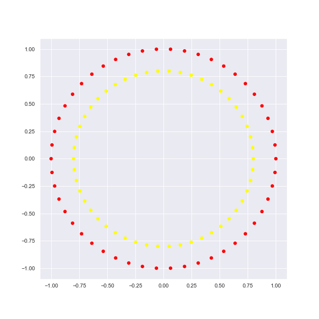
datasets.make_circles
Let’s try a simple circle dataset of sklearn. First we generate it and output its features: (x, y) coordinates and target: classifier value or label.
circles[0]contains featurescircles[1]contains values/labels.
In our case only 2 labels, namely {0, 1}.
circles = datasets.make_circles()
print("features: {}".format(circles[0][:10]))
print("target: {}".format(circles[1][:10]))
features: [[ 9.68583161e-01 2.48689887e-01] [-1.00000000e+00 -3.21624530e-16] [ 5.83174902e-01 5.47637685e-01] [ 1.87381315e-01 -9.82287251e-01] [ 5.09939192e-01 6.16410594e-01] [ 6.27905195e-02 -9.98026728e-01] [-7.93691761e-01 -1.00266587e-01] [-5.02324156e-02 7.98421383e-01] [ 7.93691761e-01 -1.00266587e-01] [ 5.35826795e-01 8.44327926e-01]]
target: [0 0 1 0 1 0 1 1 1 0]
We use the ListedColormap. It is a colormap object generated from a list of colors.
from matplotlib.colors import ListedColormap
colors = ListedColormap(['red', 'yellow'])
We use pyplot.scatter that plots of y vs x with varying marker size and/or color. First we generate lists: (1) of x coordinates and (2) of y coordinates; the 3-d parameters being a label value. The 4-th parameters, cmap, is a Colormap instance.
def plot_2d_dataset(data, colors, img_name='image.png'):
    pyplot.figure(figsize(9, 9))
    pyplot.scatter(list(map(lambda x: x[0], data[0])), list(map(lambda x: x[1], data[0])), c = data[1], cmap = colors)
    pyplot.savefig(
        img_name,
        format='png',
        dpi=72
    )
plot_2d_dataset(circles, colors, 'circles-2.png')
Noise addition
Let’s add some noise to the circles dataset.
noisy_circles = datasets.make_circles(noise = 0.15) # 15% of noise
plot_2d_dataset(noisy_circles, colors,  'circles-2-with-noise.png')
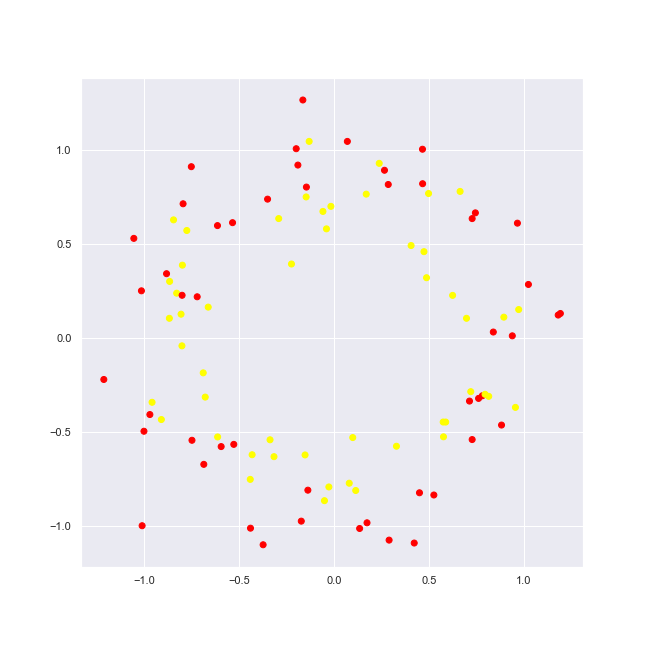
We see now really new picture, yet still one may dissern items of 2 circles.
datasets.make_classification
We take now the dataset function that allows us to generate a random n-class classification problem. It’s characterisises with the following:
- The informative, redundant and repeated features
- The [number of] classes (or labels) of the classification problem
- more parameters
simple_classification_problem = datasets.make_classification( \
    n_features = 2,  n_informative = 1, n_redundant = 1, \
    n_clusters_per_class = 1, random_state = 1 )
plot_2d_dataset(simple_classification_problem, colors,  'simple-classification.png')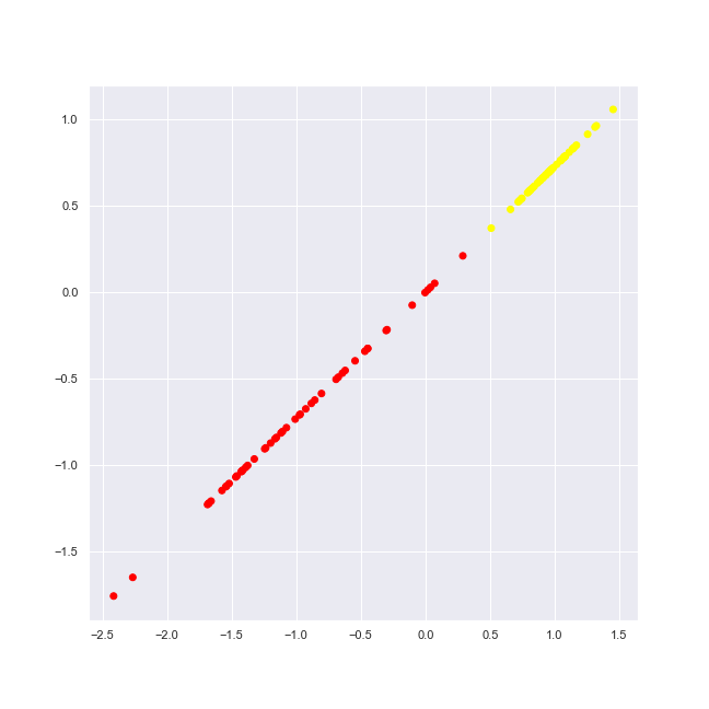
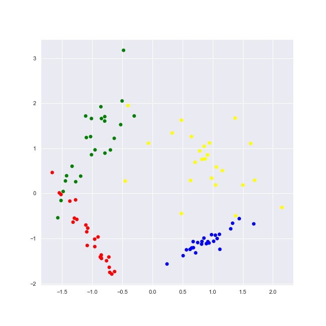
We generate dataset with 2 informative features, 4 classes (labels).
random_state=1 determines random number generation for dataset creation, dataset being reproducible across multiple function calls.
classification_problem = datasets.make_classification(n_features = 2, n_informative = 2, n_classes = 4,  n_redundant = 0, n_clusters_per_class = 1, random_state = 1)
colors = ListedColormap(['red', 'blue', 'green', 'yellow'])
As we plot it, we may observe the 4 [distinctive] classes.
plot_2d_dataset(classification_problem, colors, 'classification-2-features-4-classes.png')
“Toy” datasets
The sklearn Python module provides some well-known datasets to play with. Among them are the following:
- load_iris
- load_boston
- load_diabetes
- load_digits
- load_linnerud
datasets.load_iris
iris = datasets.load_iris()
One may easily view all of the dataset keys and get info based on them.
iris.keys()
dict_keys(['data', 'target', 'frame', 'target_names',
 'DESCR', 'feature_names', 'filename'])
One of them being DESCR key, letting us to see a dataset description.
print(iris.DESCR)
.. _iris_dataset:
Iris plants dataset
--------------------
**Data Set Characteristics:**
    :Number of Instances: 150 (50 in each of three classes)
    :Number of Attributes: 4 numeric, predictive attributes and the class
    :Attribute Information:
        - sepal length in cm
        - sepal width in cm
        - petal length in cm
        - petal width in cm
        - class:
                - Iris-Setosa
                - Iris-Versicolour
                - Iris-Virginica
    :Summary Statistics:
    ============== ==== ==== ======= ===== ====================
                    Min  Max   Mean    SD   Class Correlation
    ============== ==== ==== ======= ===== ====================
    sepal length:   4.3  7.9   5.84   0.83    0.7826
    sepal width:    2.0  4.4   3.05   0.43   -0.4194
    petal length:   1.0  6.9   3.76   1.76    0.9490  (high!)
    petal width:    0.1  2.5   1.20   0.76    0.9565  (high!)
    ============== ==== ==== ======= ===== ====================
    :Missing Attribute Values: None
    :Class Distribution: 33.3% for each of 3 classes.
    :Creator: R.A. Fisher
    :Donor: Michael Marshall (MARSHALL%PLU@io.arc.nasa.gov)
    :Date: July, 1988
The famous Iris database, first used by Sir R.A. Fisher. The dataset is taken
from Fisher's paper. Note that it's the same as in R, but not as in the UCI
Machine Learning Repository, which has two wrong data points.
This is perhaps the best known database to be found in the
pattern recognition literature.  Fisher's paper is a classic in the field and
is referenced frequently to this day.  (See Duda & Hart, for example.)  The
data set contains 3 classes of 50 instances each, where each class refers to a
type of iris plant.  One class is linearly separable from the other 2; the
latter are NOT linearly separable from each other.
.. topic:: References
   - Fisher, R.A. "The use of multiple measurements in taxonomic problems"
     Annual Eugenics, 7, Part II, 179-188 (1936); also in "Contributions to
     Mathematical Statistics" (John Wiley, NY, 1950).
   - Duda, R.O., & Hart, P.E. (1973) Pattern Classification and Scene Analysis.
     (Q327.D83) John Wiley & Sons.  ISBN 0-471-22361-1.  See page 218.
   - Dasarathy, B.V. (1980) "Nosing Around the Neighborhood: A New System
     Structure and Classification Rule for Recognition in Partially Exposed
     Environments".  IEEE Transactions on Pattern Analysis and Machine
     Intelligence, Vol. PAMI-2, No. 1, 67-71.
   - Gates, G.W. (1972) "The Reduced Nearest Neighbor Rule".  IEEE Transactions
     on Information Theory, May 1972, 431-433.
   - See also: 1988 MLC Proceedings, 54-64.  Cheeseman et al"s AUTOCLASS II
     conceptual clustering system finds 3 classes in the data.
   - Many, many more ...
We see below 4 featues and 3 classes of the iris dataset.
print("feature names: {}".format(iris.feature_names))
print("target names: {names}".format(names = iris.target_names))
feature names: ['sepal length (cm)', 'sepal width (cm)',
'petal length (cm)', 'petal width (cm)']
target names: ['setosa' 'versicolor' 'virginica']
iris.data[:10]
array([[5.1, 3.5, 1.4, 0.2],
       [4.9, 3. , 1.4, 0.2],
       [4.7, 3.2, 1.3, 0.2],
       [4.6, 3.1, 1.5, 0.2],
       [5. , 3.6, 1.4, 0.2],
       [5.4, 3.9, 1.7, 0.4],
       [4.6, 3.4, 1.4, 0.3],
       [5. , 3.4, 1.5, 0.2],
       [4.4, 2.9, 1.4, 0.2],
       [4.9, 3.1, 1.5, 0.1]])
iris.target
array([0, 0, 0, 0, 0, 0, 0, 0, 0, 0, 0, 0, 0, 0, 0, 0, 0, 0, 0, 0, 0, 0,
       0, 0, 0, 0, 0, 0, 0, 0, 0, 0, 0, 0, 0, 0, 0, 0, 0, 0, 0, 0, 0, 0,
       0, 0, 0, 0, 0, 0, 1, 1, 1, 1, 1, 1, 1, 1, 1, 1, 1, 1, 1, 1, 1, 1,
       1, 1, 1, 1, 1, 1, 1, 1, 1, 1, 1, 1, 1, 1, 1, 1, 1, 1, 1, 1, 1, 1,
       1, 1, 1, 1, 1, 1, 1, 1, 1, 1, 1, 1, 2, 2, 2, 2, 2, 2, 2, 2, 2, 2,
       2, 2, 2, 2, 2, 2, 2, 2, 2, 2, 2, 2, 2, 2, 2, 2, 2, 2, 2, 2, 2, 2,
       2, 2, 2, 2, 2, 2, 2, 2, 2, 2, 2, 2, 2, 2, 2, 2, 2, 2])
Visualize the iris dataset
First we load the iris dataset into a Pandas DataFrame.
from pandas import DataFrame
iris_frame = DataFrame(iris.data)
iris_frame.columns = iris.feature_names
iris_frame['target'] = iris.target
iris_frame.head()
| sepal length (cm) | sepal width (cm) | petal length (cm) | petal width (cm) | target | |
|---|---|---|---|---|---|
| 0 | 5.1 | 3.5 | 1.4 | 0.2 | 0 |
| 1 | 4.9 | 3.0 | 1.4 | 0.2 | 0 |
| 2 | 4.7 | 3.2 | 1.3 | 0.2 | 0 |
| 3 | 4.6 | 3.1 | 1.5 | 0.2 | 0 |
| 4 | 5.0 | 3.6 | 1.4 | 0.2 | 0 |
We change the class label {0, 1, 2} to its corresponsding name: {‘setosa’ ‘versicolor’ ‘virginica’} in the Pandas DataFrame.
iris_frame.target = iris_frame.target.apply(lambda x : iris.target_names[x])
iris_frame.sample(5)
#print(iris_frame.size)
| sepal length (cm) | sepal width (cm) | petal length (cm) | petal width (cm) | target |
|---|---|---|---|---|
| 7.7 | 3.0 | 6.1 | 2.3 | virginica |
| 6.0 | 3.0 | 4.8 | 1.8 | virginica |
| 6.5 | 3.0 | 5.5 | 1.8 | virginica |
| 5.7 | 3.0 | 4.2 | 1.2 | versicolor |
| 5.1 | 3.8 | 1.5 | 0.3 | setosa |
We may easily plot any target class histogram on any of its feature.
ax = iris_frame[iris_frame.target == 'setosa'].hist('sepal length (cm)')
for a in ax.flatten():
    a.set_xlabel("Length")
    a.set_ylabel("Frequency")
fig = a.get_figure()
fig.savefig('iris-histogram-1.png')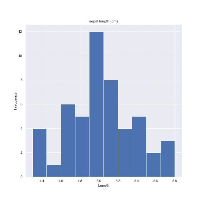
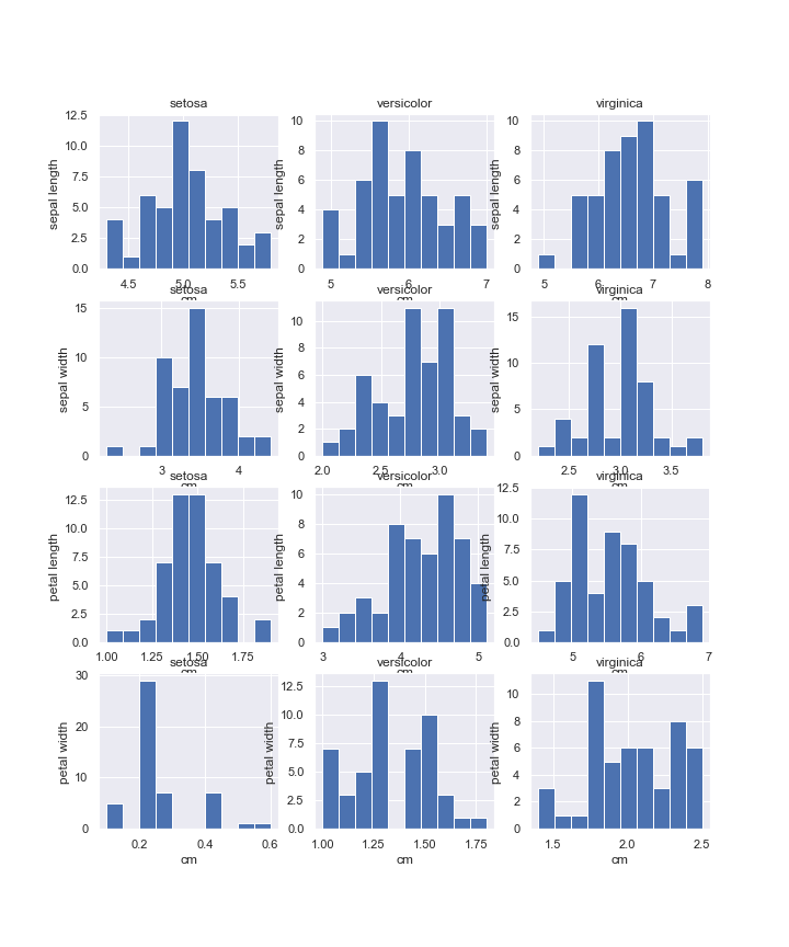
Below we plot each dataset feature (in rows) histogram for each of its targets (in columns).
pyplot.figure(figsize(10, 12))
plot_number = 0
for feature_name in iris['feature_names']:
    for target_name in iris['target_names']:
        plot_number += 1
        pyplot.subplot(4, 3, plot_number)
        pyplot.hist(iris_frame[iris_frame.target == target_name][feature_name])
        pyplot.title(target_name)
        pyplot.xlabel('cm')
        pyplot.ylabel(feature_name[:-4])
pyplot.savefig(
    'iris-targets-features-histogram-2.png',
    format='png',
    dpi=72
)
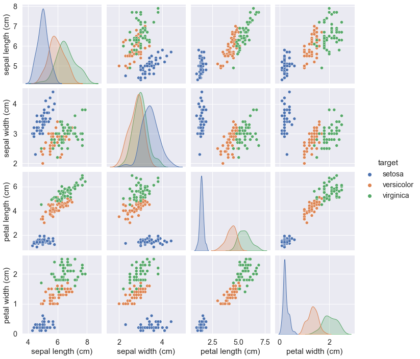
2. Seaborn library for visualization
import seaborn as sns
sns.set(font_scale = 1.3)
sns_plot = sns.pairplot(iris_frame, hue = 'target')
sns_plot.savefig("sns-plot.png")

We might get the Seaborn inbuilt dataset iris and output it too.
Note, the hue parameter should be now of “species” value.
sns.set(font_scale = 1.3)
data = sns.load_dataset("iris")
sns.pairplot(data, hue = "species")
The Seaborn library is not included into the Anaconda toolkit
So you might want to use the following:
import seaborn as sns
sns.set(font_scale = 1.3)
sns_plot = sns.pairplot(iris_frame, hue = 'target')
sns_plot.savefig("sns-plot.png")We might get the Seaborn inbuilt dataset iris and output it too.
Note, the hue parameter should be now of “species” value.
sns.set(font_scale = 1.3)
data = sns.load_dataset("iris")
sns.pairplot(data, hue = "species")
The Seaborn library is not included into the Anaconda toolkit
So you might want to use the following: